Introduction to Causal Inference: Double Machine Learning

Overview

Does a cash bonus actually cause unemployed workers to find jobs faster, or do the workers who receive bonuses simply differ from those who do not? This is the core challenge of causal inference: separating a genuine treatment effect from the confounding influence of observed and unobserved characteristics. Standard regression can adjust for covariates, but when the relationship between confounders and outcomes is complex and nonlinear, linear models may fail to fully remove bias.

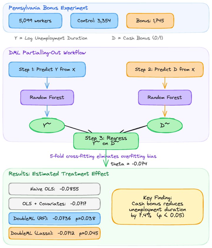
Double Machine Learning (DML) addresses this problem by using flexible machine learning models to partial out the confounding variation, then estimating the causal effect on the cleaned residuals. In this tutorial we apply DML to the Pennsylvania Bonus Experiment, a real randomized study where some unemployment insurance claimants received a cash bonus for finding employment quickly. We estimate how much the bonus reduced unemployment duration, and we compare DML estimates against naive and covariate-adjusted OLS to see how debiasing changes the results.

Learning objectives:

• Understand why prediction and causal inference require different approaches
• Learn the Partially Linear Regression (PLR) model and the partialling-out estimator
• Implement Double Machine Learning with cross-fitting using the doubleml package
• Interpret causal effect estimates, standard errors, and confidence intervals
• Assess robustness by comparing results across different ML learners

Setup and imports

Before running the analysis, install the required package if needed:

pip install doubleml

The following code imports all necessary libraries and sets the configuration variables for our analysis. We use RANDOM_SEED = 42 throughout to ensure reproducibility, and define the outcome, treatment, and covariate columns that will be used in all subsequent steps.

import numpy as np
import pandas as pd
import matplotlib.pyplot as plt
import seaborn as sns
from sklearn.base import clone
from sklearn.ensemble import RandomForestRegressor
from sklearn.linear_model import LassoCV, LinearRegression
from doubleml import DoubleMLData, DoubleMLPLR
from doubleml.datasets import fetch_bonus

# Reproducibility
RANDOM_SEED = 42
np.random.seed(RANDOM_SEED)

# Configuration
OUTCOME = "inuidur1"
OUTCOME_LABEL = "Log Unemployment Duration"
TREATMENT = "tg"
TREATMENT_LABEL = "Cash Bonus (tg)"
COVARIATES = [
    "female", "black", "othrace", "dep1", "dep2",
    "q2", "q3", "q4", "q5", "q6",
    "agelt35", "agegt54", "durable", "lusd", "husd",
]

Data loading: The Pennsylvania Bonus Experiment

The Pennsylvania Bonus Experiment is a well-known dataset in labor economics. In this study, a random subset of unemployment insurance claimants was offered a cash bonus if they found a new job within a qualifying period. The dataset records whether each claimant received the bonus offer (treatment) and how long they remained unemployed (outcome), along with demographic and labor market covariates.

df = fetch_bonus("DataFrame")

print(f"Dataset shape: {df.shape}")
print(f"Observations: {len(df)}")
print(f"\nTreatment groups:")
print(df[TREATMENT].value_counts().rename({0: "Control", 1: "Bonus"}))
print(f"\nOutcome ({OUTCOME}) summary:")
print(df[OUTCOME].describe().round(3))

Dataset shape: (5099, 26)
Observations: 5099

Treatment groups:
0    3354
1    1745
Name: tg, dtype: int64

Outcome (inuidur1) summary:
count    5099.000
mean        2.028
std         1.215
min         0.000
25%         0.693
50%         2.398
75%         3.135
max         3.950
Name: inuidur1, dtype: float64

The dataset contains 5,099 unemployment insurance claimants with 26 variables. The treatment is unevenly split: 1,745 claimants received the bonus offer while 3,354 served as controls. The outcome variable, log unemployment duration (inuidur1), ranges from 0.0 to 3.95 with a mean of 2.028 and standard deviation of 1.215, indicating substantial variation in how long claimants remained unemployed. The median (2.398) exceeds the mean, suggesting a left-skewed distribution where some claimants found jobs very quickly.

Exploratory data analysis

Outcome distribution by treatment group

Before modeling, we examine whether the outcome distributions differ visibly between treated and control groups. While a randomized experiment should produce balanced groups on average, visualizing the raw data helps us understand the structure of the outcome and spot any obvious patterns.

fig, ax = plt.subplots(figsize=(8, 5))
for group, label, color in [(0, "Control", "#6a9bcc"), (1, "Bonus", "#d97757")]:
    subset = df[df[TREATMENT] == group][OUTCOME]
    ax.hist(subset, bins=30, alpha=0.6, label=f"{label} (mean={subset.mean():.3f})",
            color=color, edgecolor="white")
ax.set_xlabel(OUTCOME_LABEL)
ax.set_ylabel("Count")
ax.set_title(f"Distribution of {OUTCOME_LABEL} by Treatment Group")
ax.legend()
plt.savefig("doubleml_outcome_by_treatment.png", dpi=300, bbox_inches="tight")
plt.show()

The histogram reveals that both groups share a similar shape, with a concentration of claimants at higher log durations (around 3.0–3.5) and a spread of shorter durations below 2.0. The bonus group shows a slightly lower mean (1.98) compared to the control group (2.05), a difference of about 0.07 log points. This raw gap hints at a potential treatment effect, but we cannot yet attribute it to the bonus because confounders may also differ between groups.

Covariate balance

In a well-designed randomized experiment, the distribution of covariates should be roughly similar across treatment and control groups. We check this balance to verify that randomization worked as expected and to understand which characteristics might confound the treatment-outcome relationship if balance is imperfect.

covariate_means = df.groupby(TREATMENT)[COVARIATES].mean()

fig, ax = plt.subplots(figsize=(12, 6))
x = np.arange(len(COVARIATES))
width = 0.35
ax.bar(x - width / 2, covariate_means.loc[0], width, label="Control",
       color="#6a9bcc", edgecolor="white")
ax.bar(x + width / 2, covariate_means.loc[1], width, label="Bonus",
       color="#d97757", edgecolor="white")
ax.set_xticks(x)
ax.set_xticklabels(COVARIATES, rotation=45, ha="right")
ax.set_ylabel("Mean Value")
ax.set_title("Covariate Balance: Control vs Bonus Group")
ax.legend()
plt.savefig("doubleml_covariate_balance.png", dpi=300, bbox_inches="tight")
plt.show()

The covariate means are nearly identical across treatment and control groups for all 15 covariates, confirming that randomization produced well-balanced groups. Demographic variables like female, black, and age indicators show negligible differences, as do the economic indicators (durable, lusd, husd). This balance is reassuring: it means that any difference in unemployment duration between groups is unlikely to be driven by observable confounders. Nevertheless, DML provides a principled way to adjust for these covariates and improve precision.

The confounding problem

Even in a randomized experiment, adjusting for covariates can improve the precision of causal estimates. In observational studies, covariate adjustment is essential to avoid confounding bias. The question is how to adjust. Standard OLS assumes a linear relationship between covariates and the outcome, which may miss complex nonlinear patterns. The naive OLS model regresses the outcome $Y$ directly on the treatment $D$:

$$Y_i = \alpha + \beta \, D_i + \epsilon_i \quad \text{(naive, no covariates)}$$

Adding covariates $X$ linearly gives:

$$Y_i = \alpha + \beta \, D_i + X_i' \gamma + \epsilon_i \quad \text{(with covariates)}$$

In both cases, $\beta$ is the estimated treatment effect. But if the true relationship between $X$ and $Y$ is nonlinear, the linear specification may leave residual confounding in $\hat{\beta}$.

Naive OLS baseline

We start with two simple OLS regressions to establish baseline estimates: one with no covariates (naive), and one that linearly adjusts for all 15 covariates. These provide a reference point for evaluating how much DML’s flexible adjustment changes the estimated treatment effect.

# Naive OLS: no covariates
ols = LinearRegression()
ols.fit(df[[TREATMENT]], df[OUTCOME])
naive_coef = ols.coef_[0]

# OLS with covariates
ols_full = LinearRegression()
ols_full.fit(df[[TREATMENT] + COVARIATES], df[OUTCOME])
ols_full_coef = ols_full.coef_[0]

print(f"Naive OLS coefficient (no covariates): {naive_coef:.4f}")
print(f"OLS with covariates coefficient:       {ols_full_coef:.4f}")

Naive OLS coefficient (no covariates): -0.0855
OLS with covariates coefficient:       -0.0717

The naive OLS estimate is -0.0855, suggesting that the bonus is associated with an 8.6% reduction in log unemployment duration. Adding covariates shrinks the estimate to -0.0717 (7.2% reduction), indicating that part of the naive association was driven by differences in observable characteristics between groups. However, linear adjustment may not capture the full confounding structure. Double Machine Learning will use flexible ML models to more thoroughly partial out covariate effects.

What is Double Machine Learning?

The Partially Linear Regression (PLR) model

Double Machine Learning operates within the Partially Linear Regression framework. The key idea is that the outcome $Y$ depends on the treatment $D$ through a linear coefficient (the causal effect we want) plus a potentially complex, nonlinear function of covariates $X$. The PLR model consists of two structural equations:

$$Y = D \, \theta_0 + g_0(X) + \varepsilon, \quad E[\varepsilon \mid D, X] = 0$$

$$D = m_0(X) + V, \quad E[V \mid X] = 0$$

Here, $\theta_0$ is the causal parameter of interest, $g_0(\cdot)$ is the nuisance function that captures how covariates affect the outcome, and $m_0(\cdot)$ models how covariates predict treatment assignment. The error terms $\varepsilon$ and $V$ are orthogonal to the covariates by construction. The challenge is that both $g_0$ and $m_0$ can be arbitrarily complex — DML uses machine learning to estimate them flexibly.

The partialling-out estimator

The DML algorithm works in two stages. First, it uses ML models to predict the outcome from covariates alone (estimating $E[Y \mid X]$) and to predict the treatment from covariates alone (estimating $E[D \mid X]$). Then it computes residuals from both predictions — the part of $Y$ not explained by $X$, and the part of $D$ not explained by $X$:

$$\tilde{Y} = Y - \hat{g}_0(X) = Y - \hat{E}[Y \mid X]$$

$$\tilde{D} = D - \hat{m}_0(X) = D - \hat{E}[D \mid X]$$

Finally, it regresses the outcome residuals on the treatment residuals to obtain the causal estimate:

$$\hat{\theta}_0 = \left( \frac{1}{N} \sum_{i=1}^{N} \tilde{D}_i^2 \right)^{-1} \frac{1}{N} \sum_{i=1}^{N} \tilde{D}_i \, \tilde{Y}_i$$

This “cleaning” step removes confounding variation, leaving only the causal relationship between $D$ and $Y$.

Cross-fitting: why it matters

A naive implementation of partialling-out would use the same data to fit the ML models and compute residuals, introducing regularization bias. DML solves this with cross-fitting: the data is split into $K$ folds, and each fold’s residuals are computed using ML models trained on the other $K-1$ folds. The cross-fitted estimator is:

$$\hat{\theta}_0^{CF} = \left( \frac{1}{N} \sum_{k=1}^{K} \sum_{i \in I_k} \left(\tilde{D}_i^{(k)}\right)^2 \right)^{-1} \frac{1}{N} \sum_{k=1}^{K} \sum_{i \in I_k} \tilde{D}_i^{(k)} \, \tilde{Y}_i^{(k)}$$

where $\tilde{Y}_i^{(k)}$ and $\tilde{D}_i^{(k)}$ are residuals for observation $i$ in fold $k$, computed using models trained on all folds except $k$. This ensures that the residuals are computed out-of-sample, eliminating overfitting bias and preserving valid statistical inference (standard errors, p-values, confidence intervals).

Setting up DoubleML

The doubleml package provides a clean interface for implementing DML. We first wrap our data into a DoubleMLData object that specifies the outcome, treatment, and covariate columns. Then we configure the ML learners: Random Forest regressors for both the outcome model ml_l (estimating $\hat{g}_0$) and the treatment model ml_m (estimating $\hat{m}_0$).

# Prepare data for DoubleML
dml_data = DoubleMLData(df, y_col=OUTCOME, d_cols=TREATMENT, x_cols=COVARIATES)
print(dml_data)

================== DoubleMLData Object ==================

------------------ Data summary      ------------------
Outcome variable: inuidur1
Treatment variable(s): ['tg']
Covariates: ['female', 'black', 'othrace', 'dep1', 'dep2', 'q2', 'q3', 'q4', 'q5', 'q6', 'agelt35', 'agegt54', 'durable', 'lusd', 'husd']
Instrument variable(s): None
No. Observations: 5099

The DoubleMLData object confirms our setup: inuidur1 as the outcome, tg as the treatment, and all 15 covariates registered. The object reports 5,099 observations and no instrumental variables, which is correct for the PLR model.

Now we configure the ML learners. We use Random Forest with 500 trees, max depth of 5, and sqrt feature sampling – a moderate configuration that balances flexibility with regularization.

# Configure ML learners
learner = RandomForestRegressor(n_estimators=500, max_features="sqrt",
                                max_depth=5, random_state=RANDOM_SEED)
ml_l_rf = clone(learner)  # Learner for E[Y|X]
ml_m_rf = clone(learner)  # Learner for E[D|X]

print(f"ml_l (outcome model): {type(ml_l_rf).__name__}")
print(f"ml_m (treatment model): {type(ml_m_rf).__name__}")
print(f"  n_estimators={learner.n_estimators}, max_depth={learner.max_depth}, max_features='{learner.max_features}'")

ml_l (outcome model): RandomForestRegressor
ml_m (treatment model): RandomForestRegressor
  n_estimators=500, max_depth=5, max_features='sqrt'

Both the outcome and treatment models use RandomForestRegressor with 500 estimators and max depth 5. The clone() function creates independent copies so that each model is trained separately during the DML fitting process. The max_features='sqrt' setting means each split considers only the square root of 15 covariates (about 4 features), adding randomness that reduces overfitting.

Fitting the PLR model

With data and learners configured, we fit the Partially Linear Regression model using 5-fold cross-fitting. The DoubleMLPLR class handles the full DML pipeline: splitting data into folds, fitting ML models on training folds, computing out-of-sample residuals, and estimating the causal coefficient with valid standard errors.

np.random.seed(RANDOM_SEED)
dml_plr_rf = DoubleMLPLR(dml_data, ml_l_rf, ml_m_rf, n_folds=5)
dml_plr_rf.fit()

print(dml_plr_rf.summary)

       coef   std err         t     P>|t|     2.5 %    97.5 %
tg -0.0736    0.0354    -2.077     0.0378   -0.1430   -0.0041

The DML estimate with Random Forest learners yields a treatment coefficient of -0.0736 with a standard error of 0.0354. The t-statistic is -2.077, producing a p-value of 0.0378, which is statistically significant at the 5% level. The 95% confidence interval is [-0.1430, -0.0041], meaning we are 95% confident that the true causal effect of the bonus lies between a 14.3% and 0.4% reduction in log unemployment duration.

Interpreting the results

Let us extract and interpret the key quantities from the fitted model to understand both the statistical and practical significance of the estimated treatment effect.

rf_coef = dml_plr_rf.coef[0]
rf_se = dml_plr_rf.se[0]
rf_pval = dml_plr_rf.pval[0]
rf_ci = dml_plr_rf.confint().values[0]

print(f"Coefficient (theta_0):  {rf_coef:.4f}")
print(f"Standard Error:         {rf_se:.4f}")
print(f"p-value:                {rf_pval:.4f}")
print(f"95% CI:                 [{rf_ci[0]:.4f}, {rf_ci[1]:.4f}]")
print(f"\nInterpretation:")
print(f"  The bonus reduces log unemployment duration by {abs(rf_coef):.4f}.")
print(f"  This corresponds to approximately a {abs(rf_coef)*100:.1f}% reduction.")
print(f"  We are 95% confident the true effect lies between")
print(f"  {abs(rf_ci[1])*100:.1f}% and {abs(rf_ci[0])*100:.1f}% reduction.")

Coefficient (theta_0):  -0.0736
Standard Error:         0.0354
p-value:                0.0378
95% CI:                 [-0.1430, -0.0041]

Interpretation:
  The bonus reduces log unemployment duration by 0.0736.
  This corresponds to approximately a 7.4% reduction.
  We are 95% confident the true effect lies between
  0.4% and 14.3% reduction.

The estimated causal effect is $\hat{\theta}_0 = -0.0736$, meaning the cash bonus reduces log unemployment duration by approximately 7.4%. Since the outcome is in log scale, this translates to roughly a 7.1% proportional reduction in actual unemployment duration (using $e^{-0.0736} - 1 \approx -0.071$). The effect is statistically significant ($p = 0.0378$), and the 95% confidence interval is constructed as:

$$\text{CI}_{95\%} = \hat{\theta}_0 \pm 1.96 \times \text{SE}(\hat{\theta}_0) = -0.0736 \pm 1.96 \times 0.0354 = [-0.1430, \; -0.0041]$$

The interval excludes zero, confirming that the bonus has a genuine causal impact. However, the wide interval — spanning from a 0.4% to 14.3% reduction — reflects meaningful uncertainty about the exact magnitude.

Sensitivity: does the choice of ML learner matter?

A key advantage of DML is that it is agnostic to the choice of ML learner, as long as the learner is flexible enough to approximate the true confounding function. To verify that our results are not driven by the specific choice of Random Forest, we re-estimate the model using Lasso (L1-regularized linear regression), a fundamentally different class of learner.

ml_l_lasso = LassoCV()
ml_m_lasso = LassoCV()

np.random.seed(RANDOM_SEED)
dml_plr_lasso = DoubleMLPLR(dml_data, ml_l_lasso, ml_m_lasso, n_folds=5)
dml_plr_lasso.fit()

print(dml_plr_lasso.summary)

       coef   std err         t     P>|t|     2.5 %    97.5 %
tg -0.0712    0.0354    -2.009     0.0445   -0.1406   -0.0018

The Lasso-based DML estimate is -0.0712 with a standard error of 0.0354 and p-value of 0.0445. This is remarkably close to the Random Forest estimate of -0.0736, with a difference of only 0.0024 – less than 7% of the standard error. The 95% confidence interval is [-0.1406, -0.0018], which also excludes zero. The near-identical results across two fundamentally different learners strongly support the robustness of the estimated treatment effect.

Comparing all estimates

To see how different estimation strategies affect the results, we visualize all four coefficient estimates side by side: naive OLS, OLS with covariates, DML with Random Forest, and DML with Lasso. The DML estimates include confidence intervals derived from valid statistical inference.

lasso_coef = dml_plr_lasso.coef[0]
lasso_se = dml_plr_lasso.se[0]
lasso_ci = dml_plr_lasso.confint().values[0]

fig, ax = plt.subplots(figsize=(8, 5))
methods = ["Naive OLS", "OLS + Covariates", "DoubleML (RF)", "DoubleML (Lasso)"]
coefs = [naive_coef, ols_full_coef, rf_coef, lasso_coef]
colors = ["#999999", "#666666", "#6a9bcc", "#d97757"]

ax.barh(methods, coefs, color=colors, edgecolor="white", height=0.6)
ax.errorbar(rf_coef, 2, xerr=[[rf_coef - rf_ci[0]], [rf_ci[1] - rf_coef]],
            fmt="none", color="#141413", capsize=5, linewidth=2)
ax.errorbar(lasso_coef, 3, xerr=[[lasso_coef - lasso_ci[0]], [lasso_ci[1] - lasso_coef]],
            fmt="none", color="#141413", capsize=5, linewidth=2)
ax.axvline(0, color="black", linewidth=0.5, linestyle="--")
ax.set_xlabel("Estimated Coefficient (Effect on Log Unemployment Duration)")
ax.set_title("Naive OLS vs Double Machine Learning Estimates")
plt.savefig("doubleml_coefficient_comparison.png", dpi=300, bbox_inches="tight")
plt.show()

All four methods agree on the direction and approximate magnitude of the treatment effect: the bonus reduces unemployment duration. The naive OLS estimate (-0.0855) is the largest in absolute terms, while covariate adjustment and DML both shrink it toward -0.07. The DML estimates with Random Forest (-0.0736) and Lasso (-0.0712) cluster closely together and fall between the two OLS benchmarks. Crucially, only the DML estimates come with valid confidence intervals, both of which exclude zero, providing statistical evidence that the effect is real.

Confidence intervals

To better visualize the uncertainty around the DML estimates, we plot the 95% confidence intervals for both the Random Forest and Lasso specifications. If both intervals are similar and exclude zero, this strengthens our confidence in the causal conclusion.

fig, ax = plt.subplots(figsize=(8, 4))
y_pos = [0, 1]
labels = ["DoubleML (Random Forest)", "DoubleML (Lasso)"]
point_estimates = [rf_coef, lasso_coef]
ci_low = [rf_ci[0], lasso_ci[0]]
ci_high = [rf_ci[1], lasso_ci[1]]

for i, (est, lo, hi, label) in enumerate(zip(point_estimates, ci_low, ci_high, labels)):
    ax.plot([lo, hi], [i, i], color="#6a9bcc" if i == 0 else "#d97757", linewidth=3)
    ax.plot(est, i, "o", color="#141413", markersize=8, zorder=5)
    ax.text(hi + 0.005, i, f"{est:.4f} [{lo:.4f}, {hi:.4f}]", va="center", fontsize=9)

ax.axvline(0, color="black", linewidth=0.5, linestyle="--")
ax.set_yticks(y_pos)
ax.set_yticklabels(labels)
ax.set_xlabel("Treatment Effect Estimate (95% CI)")
ax.set_title("Confidence Intervals: DoubleML Estimates")
plt.savefig("doubleml_confint.png", dpi=300, bbox_inches="tight")
plt.show()

Both confidence intervals are nearly identical in width and position, spanning from roughly -0.14 to near zero. The Random Forest interval [-0.1430, -0.0041] and Lasso interval [-0.1406, -0.0018] both exclude zero, but just barely – the upper bounds are very close to zero (0.4% and 0.2% reduction, respectively). This tells us that while the bonus has a statistically significant negative effect on unemployment duration, the effect size is modest and estimated with considerable uncertainty.

Summary table

Method	Coefficient	Std Error	p-value	95% CI
Naive OLS	-0.0855	–	–	–
OLS + Covariates	-0.0717	–	–	–
DoubleML (RF)	-0.0736	0.0354	0.0378	[-0.1430, -0.0041]
DoubleML (Lasso)	-0.0712	0.0354	0.0445	[-0.1406, -0.0018]

The summary table confirms a consistent pattern across all four estimation methods. The naive OLS overestimates the effect at -0.0855 because it does not adjust for confounders. Adding linear covariate controls reduces the estimate to -0.0717, and the two DML specifications produce very similar estimates of -0.0736 and -0.0712. Both DML p-values are below 0.05, providing statistically significant evidence of a causal effect. The standard errors are identical (0.0354), which is expected since both use the same sample size and cross-fitting structure.

Discussion

The Pennsylvania Bonus Experiment provides a clear demonstration of Double Machine Learning in action. Because the experiment was randomized, the DML estimates are close to the OLS estimates — the confounding function $g_0(X)$ is relatively flat when treatment assignment is independent of covariates. This is actually reassuring: in a well-designed experiment, flexible covariate adjustment should not dramatically change the results, and indeed the DML estimates ($\hat{\theta}_0 = -0.0736, -0.0712$) are close to the covariate-adjusted OLS (-0.0717).

The key finding is that the cash bonus reduces log unemployment duration by approximately 7.4%, and this effect is statistically significant (p < 0.05). In practical terms, this means the bonus incentive helped claimants find new jobs somewhat faster. However, the wide confidence intervals suggest that the true effect could be as small as 0.4% or as large as 14.3%, so policymakers should be cautious about the precise magnitude.

The robustness across learners (Random Forest vs. Lasso) is a strength of DML. Both learners capture similar confounding structure, and the near-identical estimates provide evidence that the result is not an artifact of a particular modeling choice.

Summary and next steps

This tutorial demonstrated Double Machine Learning for causal inference using the Pennsylvania Bonus Experiment. The key takeaways are:

• DML separates causal estimation from nuisance function estimation, allowing flexible ML models to handle confounders
• Cross-fitting eliminates regularization bias, enabling valid statistical inference
• The bonus reduces log unemployment duration by ~7.4% (p = 0.038), a modest but statistically significant effect
• Results are robust across Random Forest and Lasso learners, with nearly identical estimates

Limitations:

• The Pennsylvania Bonus Experiment is a randomized trial, which is the easiest setting for causal inference. DML’s advantages are more pronounced in observational studies where confounding is severe
• We used the PLR model, which assumes a linear treatment effect ($\theta_0$ is constant). More complex treatment heterogeneity could be explored with the Interactive Regression Model (IRM)
• The confidence intervals are wide, reflecting limited sample size and moderate signal strength
• We did not explore heterogeneous treatment effects (e.g., does the bonus work differently for men vs. women?)

Next steps:

• Apply DML to an observational dataset where confounding is more severe
• Explore the Interactive Regression Model for binary treatments
• Investigate treatment effect heterogeneity using DoubleML’s cate() functionality
• Compare additional ML learners (gradient boosting, neural networks)

Exercises

1. Change the number of folds. Re-run the DML analysis with n_folds=3 and n_folds=10. How do the estimates and standard errors change? What are the tradeoffs of using more vs. fewer folds?

2. Try a different ML learner. Replace the Random Forest with GradientBoostingRegressor from scikit-learn. Does the estimated treatment effect change? Compare the result to the RF and Lasso estimates.

3. Investigate heterogeneous effects. Split the sample by gender (female) and estimate the DML treatment effect separately for men and women. Is the bonus more effective for one group? What might explain any differences?

References

1. DoubleML – Python Documentation
2. Chernozhukov, V., Chetverikov, D., Demirer, M., Duflo, E., Hansen, C., Newey, W., & Robins, J. (2018). Double/Debiased Machine Learning for Treatment and Structural Parameters. The Econometrics Journal, 21(1), C1–C68.
3. Pennsylvania Bonus Experiment Dataset – DoubleML
4. scikit-learn – RandomForestRegressor
5. scikit-learn – LassoCV