Causal Inference with DoWhy

Did job training raise earnings? Model · Identify · Estimate · Refute

$1,620doubly robust ATE

$62placebo collapse

5methods agree

Carlos Mendez

Nagoya University (GSID)

June 11, 2026

The Tension

Act I

Trained workers out-earned controls by $1,794 — but did training cause it?

185 disadvantaged workers got job training; 260 did not. The trained group earned $1,794 more in 1978.

But people who enroll may differ in age, schooling, or prior earnings. Is the gap the program — or the people?

This is the central challenge of causal inference: distinguishing a genuine treatment effect from confounding differences between groups. A raw difference-in-means answers “are the groups different?” not “did the treatment work?” The whole deck is about closing that gap.

Five disciplined estimators land near $1,620 — far below the naive $1,794

Estimated ATE across six methods. The five adjusted estimators cluster tightly; the naive difference sits highest.

Spoiler figure — the payoff we earn across the deck. Don’t explain every bar yet. Just plant two facts: the adjusted estimators agree with each other (around $1,550–$1,736), and they all sit below the naive $1,794. We come back to this picture in Act III.

One estimand, four steps, five estimators — do they agree?

• The estimand: the ATE of NSW job training on 1978 earnings
• DoWhy’s four steps — Model → Identify → Estimate → Refute
• Five estimators across three paradigms — do they agree?
• The discipline: refutation tests that try to break the result

Built from the post’s learning objectives. The throughline is DoWhy’s sequential discipline: you cannot estimate before you identify, and you cannot identify before you state assumptions.

The Investigation

Act II

We target the ATE: the effect of training on a random worker

\[\text{ATE} = E[Y(1) - Y(0)]\]

The expected earnings gain from moving anyone — treated or not — from no-training to training.

Four methods target the ATE directly; matching drifts toward the ATT (the effect on those actually trained) because it discards unmatched controls.

Name the estimand before estimating it. ATE answers “what if we trained everyone at random?”; ATT answers “what was the effect on those who enrolled?” The distinction matters because enrollees may differ systematically. We flag matching’s drift toward ATT when we get there.

DoWhy forces four explicit steps instead of one black-box regression

• Model — encode assumptions as a causal graph (a DAG)
• Identify — graph theory finds the adjustment formula (the estimand)
• Estimate — compute the number with one or more methods
• Refute — stress-test the result with falsification tests

You cannot estimate before you identify, and you cannot identify before you model. That ordering is the contribution.

Most software jumps straight from data to a coefficient and calls it causal. DoWhy’s discipline is the sequence: assumptions first, formula second, number third, stress test last. The post’s running analogy: build the bridge, check it stands, drive a truck across, then earthquake-test it.

The lab: 445 NSW workers, 8 pre-treatment covariates, randomized

• Outcome — real earnings in 1978 (re78), mean $5,301, heavily right-skewed
• Treatment — randomized job training (185 trained, 260 control)
• Covariates — age, education, race, marital status, degree, prior earnings (re74, re75)

All eight covariates are measured before treatment, so they can only be confounders — never mediators or colliders.

The Lalonde data from the National Supported Work Demonstration. Randomization gives a credible ground truth, which is why this is the benchmark dataset for testing causal estimators. The 8 pre-treatment covariates make the graph simple: every covariate points to both treatment and outcome.

Both groups overlap heavily — and both spike at zero earnings

Distribution of 1978 earnings by treatment group. Training mean $6,349 vs control $4,555; both right-skewed with a spike at zero.

The raw gap is $1,794 (6,349 − 4,555). But notice the heavy overlap and the shared spike at zero — many workers earned nothing regardless of training. A difference of means is a blunt instrument on data this skewed; that is the motivation for covariate adjustment.

Randomization isn’t perfect: nodegr is imbalanced by 0.31 SD

Love plot of absolute standardized mean differences. nodegr, hisp, and educ exceed the 0.1 balance threshold (orange); the rest are balanced (blue).

The SMD rescales every covariate to standard-deviation units, so dollars and years become comparable. Prior earnings look imbalanced in raw dollars but are fine once standardized. The real imbalances are nodegr (~0.31), hisp (~0.18), educ (~0.14) — chance imbalances from the small sample. Under randomization the naive estimate is still unbiased; adjusting mainly improves precision.

Step 1 — Model: every covariate is a common cause of both arms

DoWhy’s DAG: the eight covariates point to both treatment (treat) and outcome (re78); treat points to re78.

The graph encodes qualitative assumptions before we touch a number. Each arrow is a falsifiable claim. Because the covariates are pre-treatment, they are confounders — common causes of both treatment and outcome — so the DAG is straightforward: every covariate to both nodes, and treatment to outcome (the effect we want).

Step 2 — Identify: the backdoor criterion seals all confounding paths

\[\frac{d}{d[\text{treat}]}\, E[\text{re78} \mid \text{age}, \text{educ}, \text{black}, \dots, \text{re75}]\]

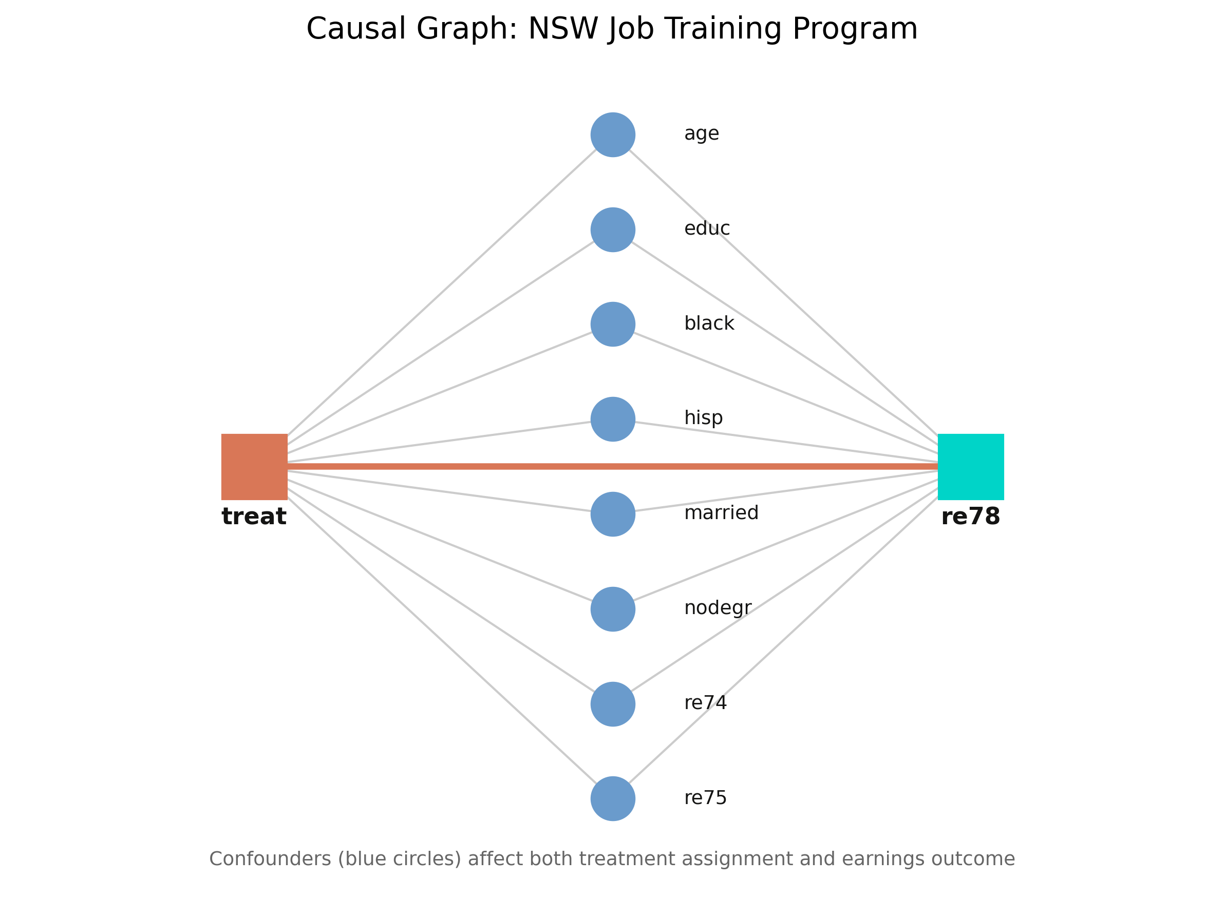
Conditioning on the eight covariates blocks every backdoor path, so the effect is identified — under unconfoundedness (no hidden common cause).

DoWhy checks backdoor, instrumental-variable, and front-door strategies automatically, and returns the formula — not a guess about what to “control for”.

Identification is the bridge between assumptions (the graph) and computation (the data). It answers “can we even compute this without a new experiment?” Here the answer is yes via backdoor adjustment, conditional on the one assumption that there is no unmeasured confounder. DoWhy automates the check, preventing the common mistake of hand-picking controls.

Step 3 — Estimate: three paradigms, one question

Outcome modeling

• Models \(E[Y \mid X, T]\)
• Regression adjustment

Treatment modeling

• Models \(P(T \mid X)\)
• IPW · stratification · matching

Doubly robust

• Models both
• AIPW

If outcome-based and treatment-based methods agree, neither model is badly misspecified — that agreement is the robustness check.

The five estimators split into three families by what they model. Outcome modeling specifies how covariates relate to earnings; treatment modeling specifies how covariates relate to assignment (the propensity score); doubly robust does both. Comparing across paradigms is powerful precisely because they fail in different ways.

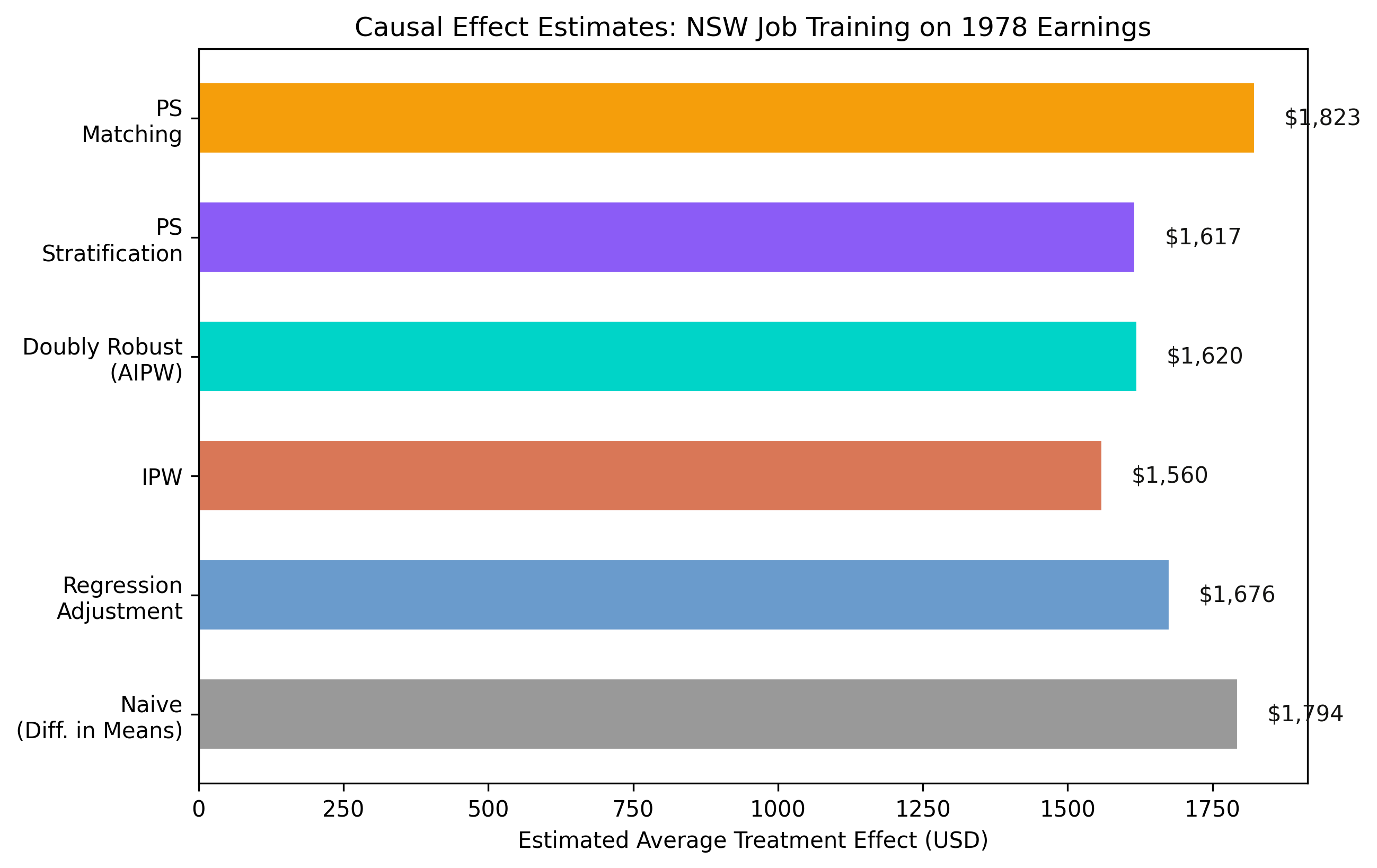
Regression adjustment compares like with like: $1,676

estimate_ra = model.estimate_effect(
    identified_estimand,
    method_name="backdoor.linear_regression",
    confidence_intervals=True)   # ATE = $1,676.34

Models \(E[Y \mid X, T]\) and reads the treatment coefficient — the gap at the same covariate values.

This is the most transparent estimator and the Frisch–Waugh–Lovell baseline: the treatment coefficient equals what you’d get by partialling out the covariates from both treatment and outcome, then regressing the residuals. It shrinks the naive $1,794 to $1,676 — about $118 of the raw gap was finite-sample imbalance, not training.

IPW re-weights surprising cases by \(1/\hat{e}(X)\): $1,559

\[\hat{\tau}_{IPW} = \frac{1}{n}\sum_{i=1}^{n}\left[\frac{T_i Y_i}{\hat{e}(X_i)} - \frac{(1-T_i)Y_i}{1-\hat{e}(X_i)}\right]\]

A treated worker who was unlikely to be treated (\(\hat{e} = 0.1\)) gets weight 10 — they are the most informative comparison.

IPW makes no assumptions about the outcome model — only that the propensity score model is right. It builds a pseudo-population where treatment is independent of covariates, mimicking a randomized experiment. Its weakness: extreme propensity scores produce huge weights and high variance. Here it gives $1,559, the lowest estimate, because it leans entirely on the treatment model.

AIPW gets two shots at the truth: $1,620

\[\hat{\tau}_{DR} = \frac{1}{n}\sum_{i=1}^{n}\left[\hat{\mu}_1(X_i) - \hat{\mu}_0(X_i) + \frac{T_i(Y_i - \hat{\mu}_1(X_i))}{\hat{e}(X_i)} - \frac{(1-T_i)(Y_i - \hat{\mu}_0(X_i))}{1-\hat{e}(X_i)}\right]\]

Consistent if either the outcome model or the propensity model is correct — belt and suspenders.

AIPW starts from regression adjustment and adds an IPW-weighted correction on the prediction errors. If the outcome model is right, the correction averages to zero; if it’s wrong but the propensity model is right, the correction fixes the bias. Only one of the two needs to be correct. It lands at $1,620, between regression ($1,676) and IPW ($1,559) — the sign that neither model is badly off.

All five adjusted estimators agree: $1,559 to $1,736

Method	Estimated ATE	What it models
Naive (diff. in means)	$1,794	nothing
Regression adjustment	$1,676	outcome
IPW	$1,559	treatment
Doubly robust (AIPW)	$1,620	both
PS stratification	$1,617	treatment
PS matching	$1,736	treatment (→ ATT)

The doubly robust $1,620 is the most credible single estimate — it survives misspecification of either model.

Convergence across fundamentally different strategies is the headline of the estimate step. Matching is the outlier at $1,736 and closest to the naive value because it discards unmatched controls — its estimand drifts toward the ATT. On a control mean of $4,555 the cluster is roughly a 34–38% earnings gain.

The Resolution

Act III

Step 4 — Refute: a placebo treatment collapses the effect to $62

$62

Placebo ATE after randomly permuting treatment (\(p = 0.92\)) — down from $1,676

The placebo refuter replaces real treatment with a random permutation. If the effect were a model artifact, it would persist; instead it falls from $1,676 to $62 — essentially zero. The high p-value (0.92) says the real estimate is far above placebo noise. This is the single most convincing test in the deck.

Add a fake confounder, drop 20% of the data — the estimate barely moves

Refutation test	New effect	p-value	Reading
Placebo treatment	$62	0.92	effect vanishes
Random common cause	$1,676	0.90	stable with noise
Data subset (80%)	$1,728	0.80	stable across subsamples

Surviving placebo, random-common-cause, and subset tests is evidence, not proof — refutation can falsify, never confirm.

Three falsification tests, three different threats: artifact (placebo), omitted confounder (random common cause), and influential observations (subset). The estimate holds across all three. The honest caveat: passing tests cannot prove causation, but failing any one would be a strong signal something is wrong.

Does machine-picked adjustment make this causal? No — one assumption still carries the weight

Objection. DoWhy automated the workflow, so the estimate must be airtight.

Response. The ATE is identified only under unconfoundedness — no hidden common cause of training and earnings. The four steps make assumptions explicit and testable; they cannot manufacture identification. Here randomization makes unconfoundedness credible; in observational data it is the load-bearing risk.

Steelman, don’t strawman. DoWhy’s value is transparency and discipline, not a guarantee. Refutation tests probe specific failure modes, but none can rule out an unobserved confounder. The post is explicit that this is a method demonstration on randomized data — the abortion–crime-style caveats apply doubly in observational settings.

The training effect is real: ~$1,620, a 34–38% earnings gain

$1,620

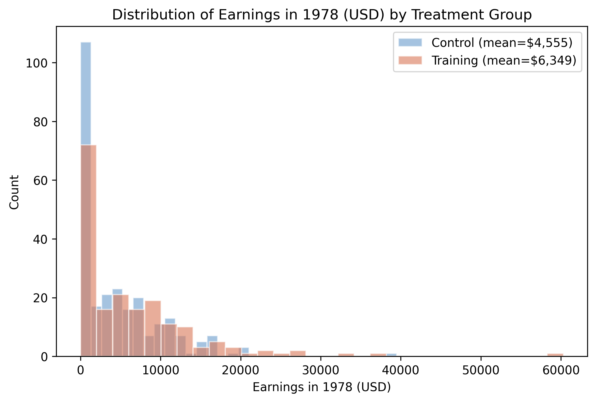
Doubly robust ATE on a control mean of $4,555 · five methods agree · refutation tests survive

The Act-III payoff and the resolution of the Act-I hook. The naive $1,794 overstated the effect by finite-sample imbalance; disciplined adjustment lands near $1,620, and the result survives every stress test. On a base of $4,555 that is a substantial 34–38% gain for a disadvantaged population.

State your assumptions, identify the estimand, then let the data — and the refutations — speak.

The single takeaway. DoWhy’s four steps don’t make causal inference automatic; they make it honest. The estimate is only as good as the unconfoundedness assumption, but Model → Identify → Estimate → Refute forces that assumption into the open where it can be argued and tested.