The FWL Theorem: Making Multivariate Regressions Intuitive

Partialling-out a confounder to recover a known +0.2 causal effect

−0.106naive slope · wrong sign

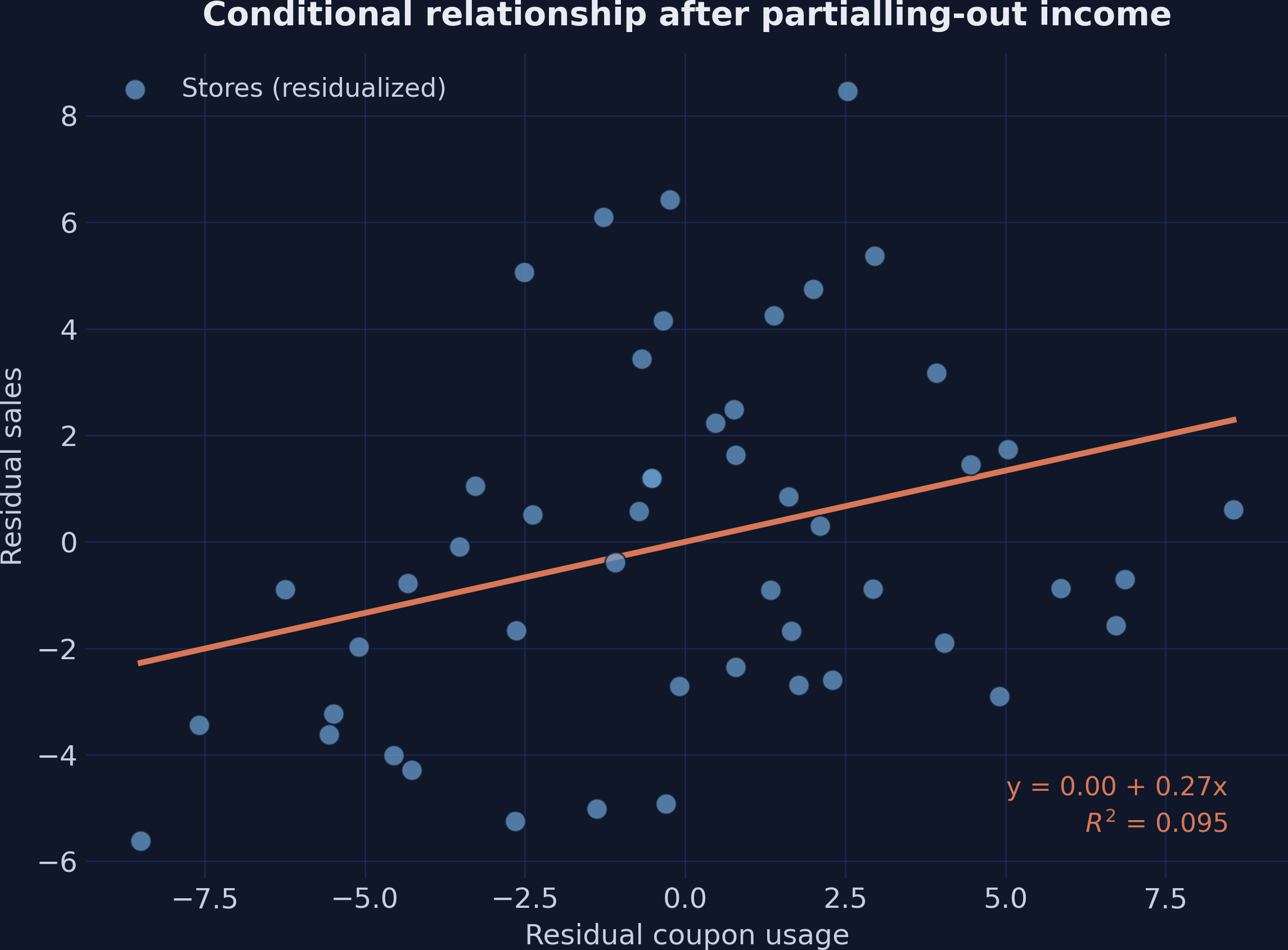
+0.267after partialling-out income

+0.200true causal effect (ATE)

Carlos Mendez

Nagoya University (GSID)

June 11, 2026

The Tension

Act I

The same coupon data says both “coupons hurt sales” and “coupons help sales”

A retail chain hands out discount coupons across 50 stores and asks one question: do the coupons increase sales?

Regress sales on coupons and the slope is negative. Add one control and it flips positive. Which answer is real?

This is the hook: a single dataset, a single question, two opposite answers. The whole deck is about why the regression changes its mind — and which version to trust. The villain is a confounder; FWL is how we see it.

Naive regression: coupons look like they reduce sales

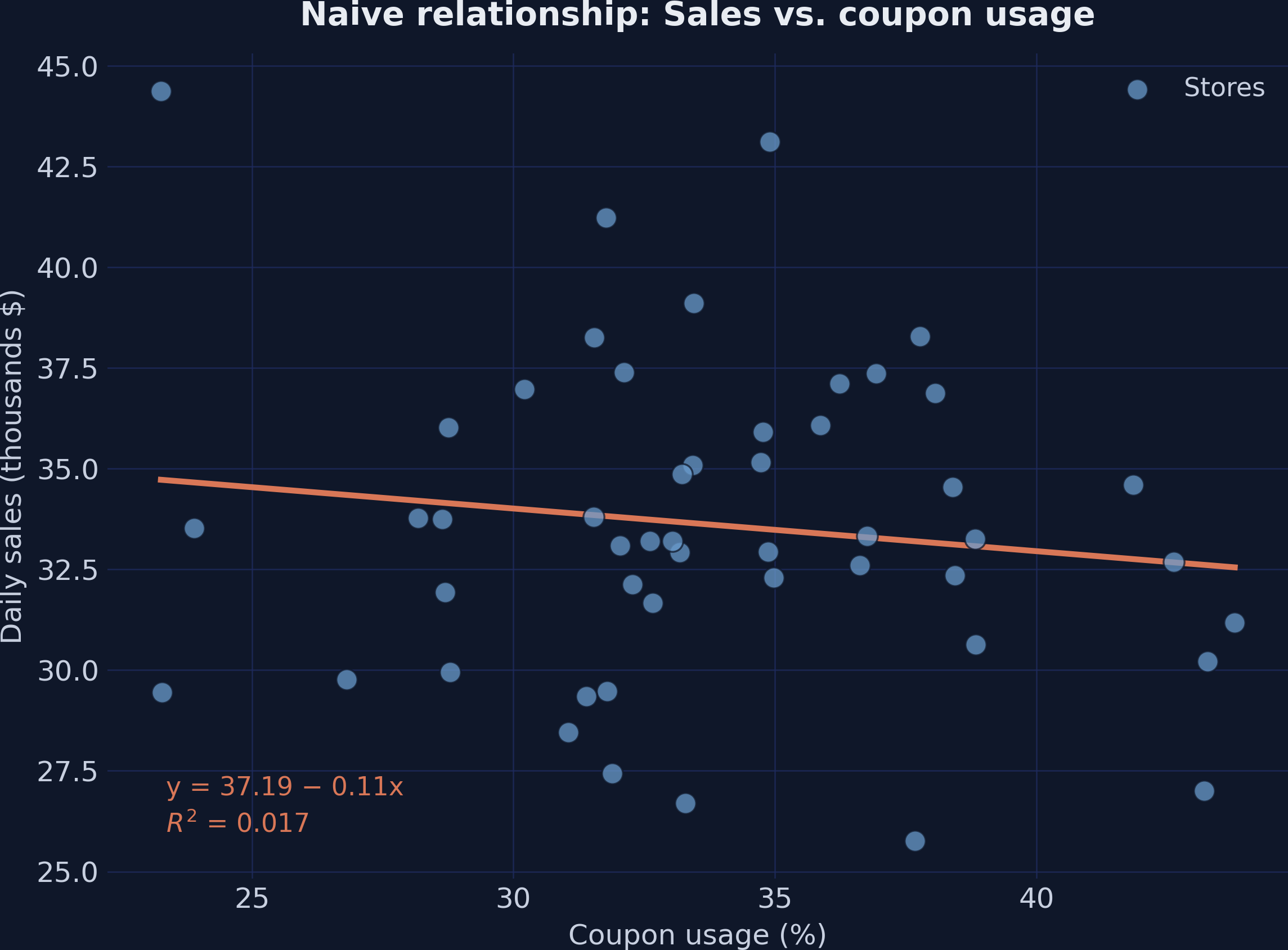
Daily sales vs. coupon usage across 50 stores. The orange fit slopes down — coupons appear to hurt sales.

Spoiler/tension figure. Don’t explain the mechanism yet — just plant that the raw picture is negative and misleading. We will earn the reversal in Act II and return to this picture in the side-by-side at the end.

Where we’re going

• The retail setup: a known +0.2 effect, confounded by income
• What “controlling for income” actually does, algebraically
• The FWL recipe: residualize, residualize, regress
• See the hidden conditional relationship as a scatter plot
• The bridge to Double Machine Learning

Built from the post’s five learning objectives. Teaching deck, so we signpost. Keep it to one breath per line.

The Investigation

Act II

Income is a confounder that opens a backdoor from coupons to sales

• Income → fewer coupons (wealthier stores use fewer)
• Income → more sales (wealthier stores spend more)
• Coupons → sales: true effect +0.2

The path coupons ← income → sales is non-causal. Leave it open and the negative income→coupon link leaks into the coupon slope.

This is the DAG from the post in words. Income drives both the treatment and the outcome — the textbook confounder. Blocking the backdoor means conditioning on income. FWL is the elegant way to do exactly that and to picture it.

A simulated lab with a known answer: the true effect is exactly +0.2

def simulate_store_data(n=50, seed=42):
    rng = np.random.default_rng(seed)
    income  = rng.normal(50, 10, n)                 # the confounder
    coupons = 60 - 0.5 * income + rng.normal(0, 5, n)   # income → fewer coupons
    sales   = (10 + 0.2 * coupons + 0.3 * income    # true effect = +0.2
               + 0.5 * dayofweek + rng.normal(0, 3, n))
    return pd.DataFrame(...)

We plant the answer (+0.2) in the data, then check whether each estimator finds it.

Why simulate? Because the true causal effect is known by construction — exactly +0.2 — so we can grade every method against ground truth. 50 stores, income centered at $50K, coupons depend negatively on income, sales depend positively on both. This is a controlled experiment inside the computer.

The naive slope is −0.106 — and points the wrong way (p = 0.365)

Model	Coupons coef.	SE	p
Naive OLS (no controls)	−0.1059	0.116	0.365

Not just imprecise — the sign is backwards from the true +0.2. The confounder is pulling it down.

Each extra percentage point of coupons is “associated with” $106 less in daily sales — but it is not significant and it contradicts the planted +0.2. Wealthy neighborhoods use fewer coupons yet spend more, so the raw slope inherits income’s negative coupon link. This is the result the controls will fix.

Add income as a control and the slope flips to +0.267 (p = 0.031)

Model	Coupons coef.	Income coef.	p
Naive OLS	−0.1059	—	0.365
Full OLS (+ income)	+0.2673	+0.3836	0.031

Conditioning on income blocks the backdoor: the estimate jumps to +0.267, close to the true +0.2.

One control reverses the conclusion. The CI [0.025, 0.509] now excludes zero. Income itself is strongly positive (+0.3836, p < 0.001), confirming richer stores spend more. But what is the regression doing when it “controls for” income? That mechanism is FWL.

FWL: any multivariate coefficient is a univariate slope on residuals

\[\hat\beta_1^{FWL}=\frac{\mathrm{Cov}(\tilde y,\ \tilde x_1)}{\mathrm{Var}(\tilde x_1)}\]

where \(\tilde x_1\) is the residual of \(x_1\) (coupons) regressed on \(x_2\) (income), and \(\tilde y\) is the residual of \(y\) (sales) regressed on \(x_2\).

Remove income from coupons, remove income from sales, then regress the leftovers. Same \(\hat\beta_1\).

Frisch & Waugh (1933), Lovell (1963). This is an algebraic identity, not an approximation. The tilde is partialling-out: keep only the variation orthogonal to income. Three equivalent estimators — full OLS, residualize-X-only, residualize-both — all return the same coefficient on coupons.

Three lines of statsmodels reproduce the multivariate coefficient

# residualize each variable with respect to income
df["coupons_tilde"] = smf.ols("coupons ~ income", df).fit().resid
df["sales_tilde"]   = smf.ols("sales ~ income",   df).fit().resid
# regress residual sales on residual coupons (no intercept)
fwl = smf.ols("sales_tilde ~ coupons_tilde - 1", df).fit()

Residuals are mean-zero, so we drop the intercept. The coefficient on coupons_tilde is the controlled effect.

The full script is in the post; these are the load-bearing lines. Step 1 residualizes only coupons and gets the right coefficient but a blown-up SE (1.271). Step 2 residualizes sales too and the SE collapses back to 0.118 — that’s why we residualize both.

Residualize-both reproduces +0.2673 exactly — and recovers the SE

FWL step	Coupons coef.	SE	p
Step 1 — residualize \(x_1\) only	+0.2673	1.271	0.834
Step 2 — residualize both	+0.2673	0.118	0.028

Same coefficient to four decimals; residualizing the outcome too restores the SE to match full OLS (0.120).

Step 1’s SE explodes because income’s variation is still sitting in sales, inflating the residual variance. Once sales is also residualized, SE = 0.118 and p = 0.028 — nearly identical to full OLS. The tiny gap is a degrees-of-freedom adjustment. FWL is exact for the point estimate.

Partialling-out, drawn: the residuals are coupon variation income can’t explain

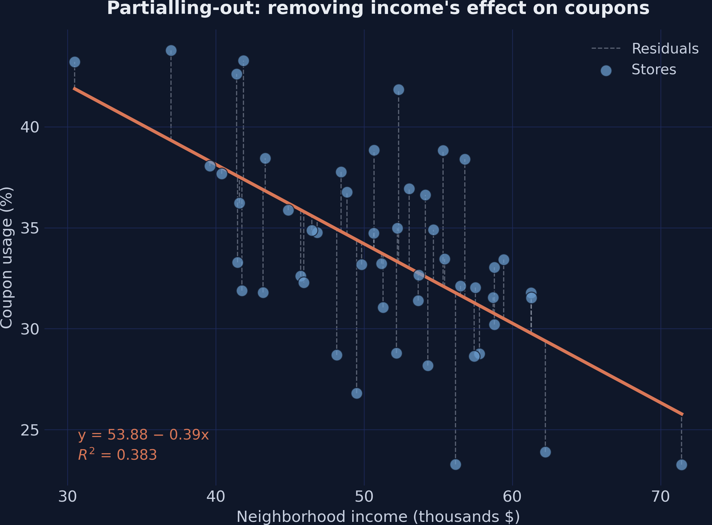
Coupon usage vs. income; the orange line is the income→coupons fit, dashed lines are the residuals each store keeps.

Look at the dashed segments first. The downward fit confirms richer stores use fewer coupons. Each dashed line is a residual — how unusual a store’s coupon use is given its income. Partialling-out throws away the line and keeps only those segments: “among similar-income stores, who couponed more or less than expected?”

The hidden positive relationship the table couldn’t show you

Residualized sales vs. residualized coupons. With income removed from both, the slope is the +0.267 conditional effect.

This is the payoff plot — the conditional relationship a multivariate regression captures but cannot draw. Stores that couponed more than expected also sold more than expected. The slope of this single line is exactly 0.2673, the full-regression coefficient, now visible to a non-technical audience.

Adding the means back keeps the slope but restores readable units

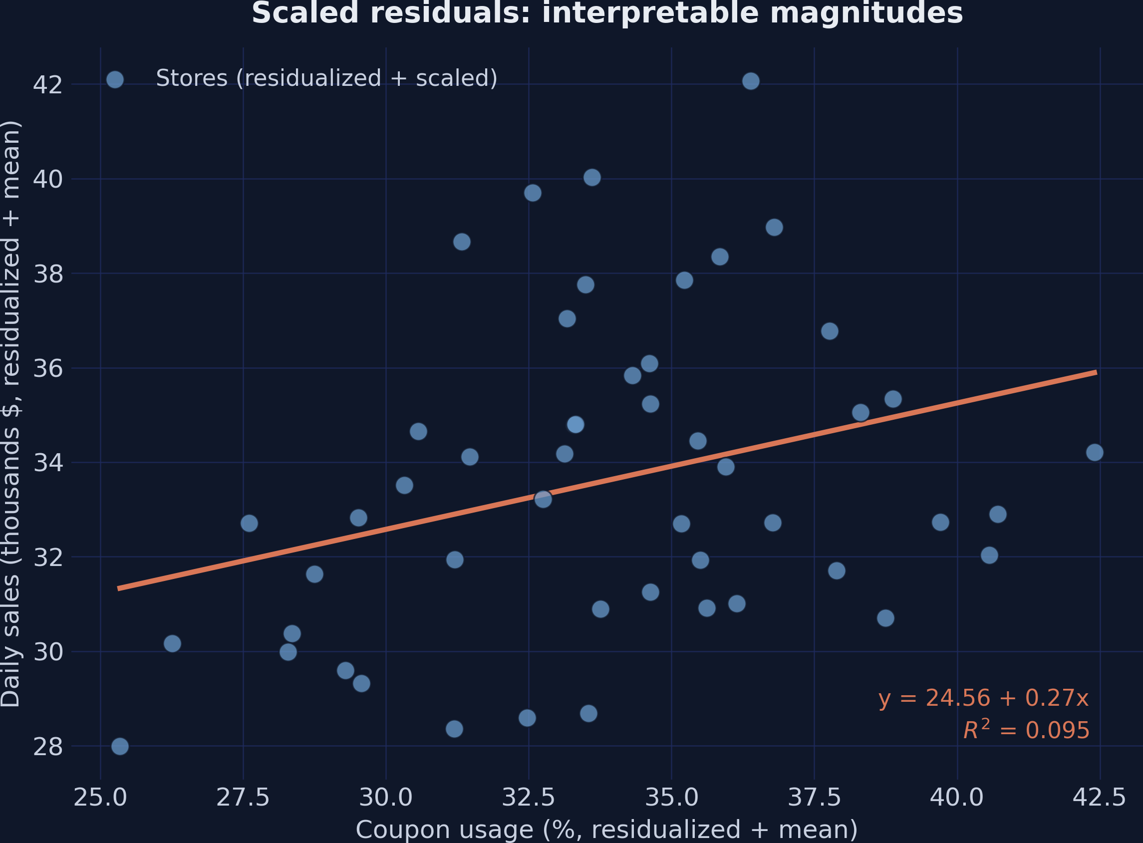
Same residual scatter shifted by the sample means — axes now read ~34% coupons and ~$33.6K sales, slope still +0.267.

A residual of −5 doesn’t mean −5% coupon usage; it means 5 points below what income predicts. Adding each variable’s mean back shifts the axes into interpretable units without touching the slope (still 0.2673, p = 0.029). This is the version for a slide or a stakeholder report.

FWL scales: two controls, same identity, +0.2706

Model	Coupons coef.	SE	p
Full OLS (+ income + day)	+0.2706	0.119	0.028
FWL (+ income + day)	+0.2706	0.116	0.023

Partial out income and day-of-week from both sides — identical coefficient. The theorem holds for any number of controls.

Day-of-week itself isn’t significant (0.3195, p = 0.198), but absorbing its variance sharpens the coupon estimate slightly, from 0.2673 to 0.2706. The FWL recipe is unchanged — residualize on the full control set, then regress. This is exactly why fixed-effects packages (reghdfe, fixest, pyfixest) partial out hundreds of dummies first.

The Resolution

Act III

After partialling-out income, coupons raise sales by +0.267

+0.267

\(\hat\beta_1\) on coupons, full OLS = FWL (SE 0.118) · matches the true +0.200 within finite-sample noise

Between the misleading naive −0.106 and the planted truth +0.200, the conditioned estimate lands at +0.267 — close, with the gap due to just 50 observations. The point: the same data, honestly conditioned, recovers the right sign and roughly the right magnitude.

Simpson’s paradox, resolved: the slope flips from −0.106 to +0.267

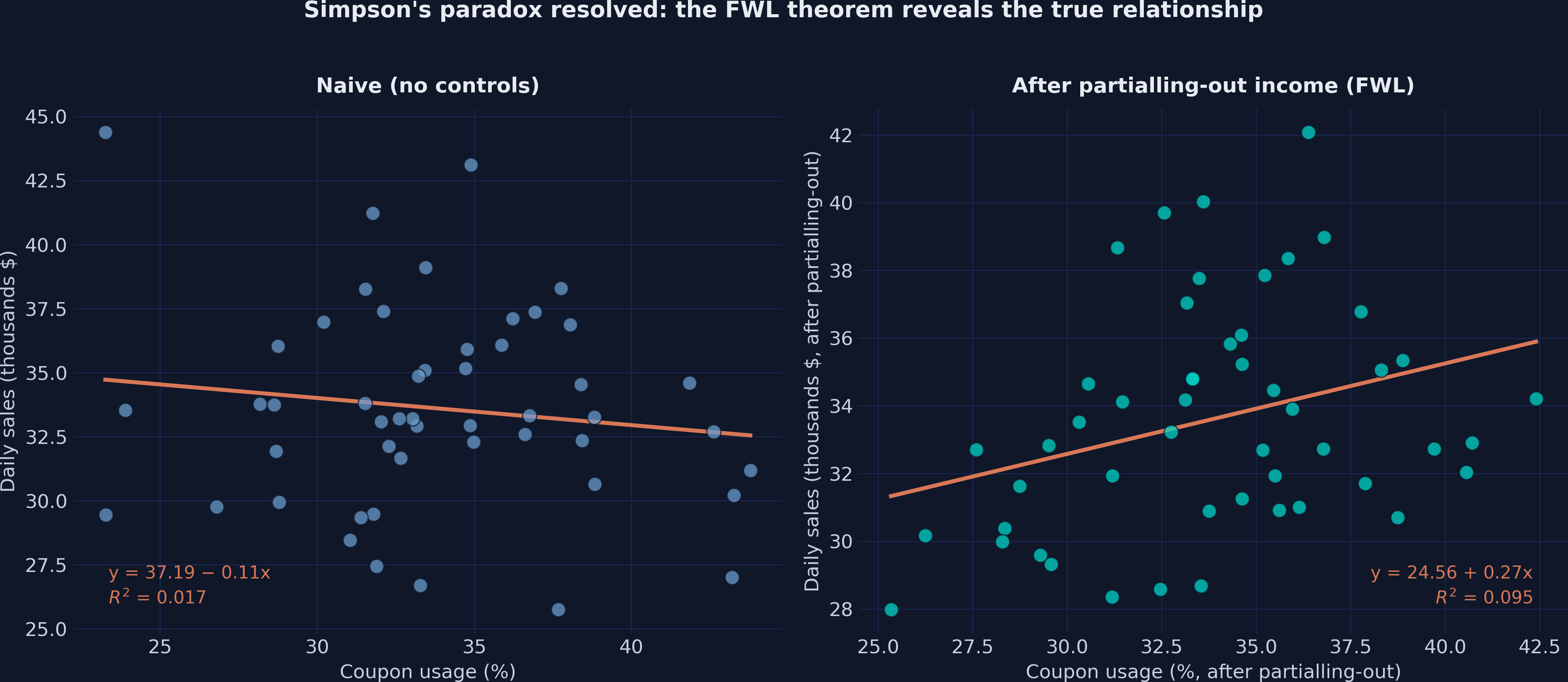
Left: naive negative slope. Right: positive slope after partialling-out income. Same 50 stores.

The single most persuasive slide. Left panel is the lie (slope −0.106), right panel is the truth (slope +0.267), and only the conditioning changed. A trend in the aggregate reverses once you condition on the relevant variable — the textbook definition of Simpson’s paradox. This is what FWL lets you draw.

Six estimators, one coefficient: FWL is an identity, not an approximation

Method	Coupons coef.	SE	p
Naive OLS (no controls)	−0.1059	0.116	0.365
Full OLS (+ income)	+0.2673	0.120	0.031
FWL residualize \(x\) only	+0.2673	1.271	0.834
FWL residualize both	+0.2673	0.118	0.028
Full OLS (+ income + day)	+0.2706	0.119	0.028
FWL (+ income + day)	+0.2706	0.116	0.023

Every FWL variant matches its full-regression twin to four decimals. The only thing that moves the coefficient is which controls you partial out, not how you do the algebra. +0.267 sits beside the true +0.200 — the difference is sampling noise in 50 stores.

Does FWL make this causal? No — it visualizes, it does not identify

Objection. Residualizing on income looks like a trick that manufactures a causal effect.

Response. FWL is pure algebra — it only reproduces what OLS already computes. The causal reading needs one assumption: income is the only confounder. FWL pictures that adjustment; it cannot certify it.

Steelman, don’t strawman. If income affects coupons or sales nonlinearly, OLS residuals won’t fully clean the confounding — that’s the linearity caveat in the post. And if a second confounder is omitted, no amount of residualizing on income saves you. FWL disciplines and pictures the adjustment; identification still comes from the DAG.

FWL is Double Machine Learning with a linear mop

FWL (here)

• residualize \(y\), \(d\) with OLS
• regress residual \(y\) on residual \(d\)
• exact for linear confounding

Double ML

• residualize \(y\), \(d\) with ML (forest, lasso)
• regress residual \(y\) on residual \(d\)
• handles non-linear, high-dim controls

Same residualize-then-regress logic; swap OLS for a flexible learner and you get a debiased causal estimate.

Chernozhukov et al. (2018). The whole DML estimator is FWL with the OLS partial-out replaced by cross-fitted machine learning. Master FWL and DML stops being mysterious — it is this same plot, learned with a smarter mop. The companion post python_doubleml runs it on a real experiment.

Don’t read the coefficient — read the partialled-out scatter.

The one sentence to remember. A multivariate coefficient is a univariate slope on residuals; FWL lets you see it, and seeing it is what turns a confounded −0.106 into an honest +0.267.