Standard Errors in Panel Data: A Beginner's Guide in Python
![]()
1. Overview
Imagine you run a regression and find that R&D spending significantly boosts firm performance, with a t-statistic of 30. Sounds like a rock-solid result. But what if that impressive t-statistic is an illusion — a consequence of using the wrong formula for your standard errors? In panel data, where the same firms are observed year after year, this is not a hypothetical worry. The repeated observations within each firm create correlation patterns that violate the assumptions behind ordinary standard errors, and ignoring these patterns can make your estimates look far more precise than they actually are.
Standard errors are the bridge between a point estimate and a statistical conclusion. If that bridge is built on the wrong assumptions, the conclusion collapses. In a classic cross-sectional regression with independent observations, conventional standard errors work well. But panel data — where firm 1 in 2015 is related to firm 1 in 2016 — breaks the independence assumption. A firm that performs well one year tends to perform well the next. Errors within the same firm are correlated, and this within-cluster correlation means conventional standard errors understate the true uncertainty surrounding your estimates.
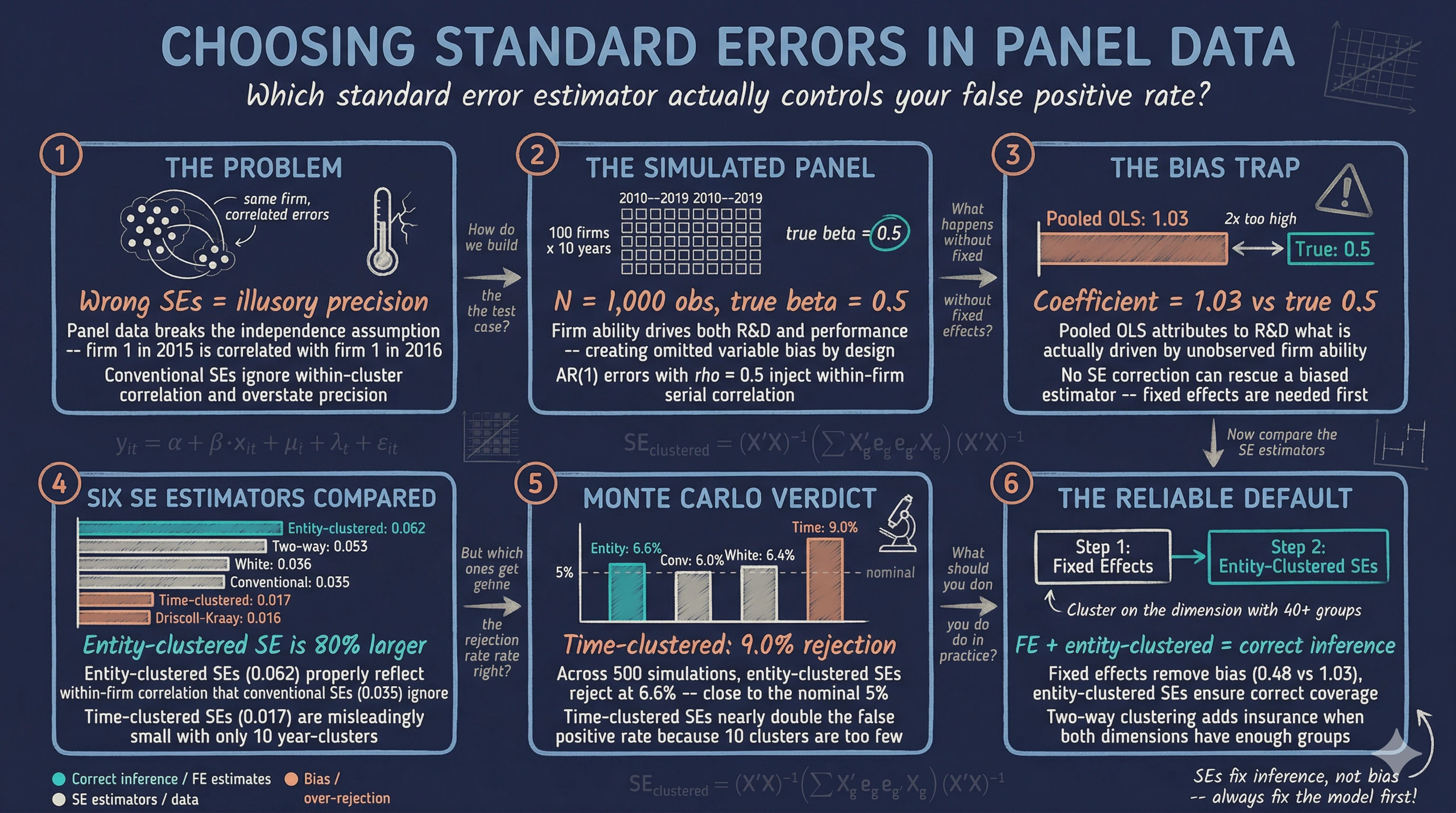
The solution is to use standard error estimators that account for the structure of the data. In this tutorial, we build a simulated panel of 100 firms over 10 years with a known true effect, then systematically compare six approaches to standard error estimation: conventional, White (heteroskedasticity-robust), entity-clustered, time-clustered, two-way clustered, and Driscoll-Kraay. Along the way, we discover two critical lessons. First, no standard error estimator can rescue a biased estimator — fixed effects are needed to remove omitted variable bias. Second, even after fixing bias, the choice of standard error estimator determines whether our confidence intervals have the coverage they promise. The tutorial is inspired by and builds upon the excellent reference by Gregoire (2024), while using original simulated data and explanations.
Learning objectives:
- Understand why within-cluster correlation invalidates conventional standard errors in panel data
- Implement six standard error estimators using Python’s
linearmodelspackage - Compare how different SE choices affect t-statistics and inference for the same regression
- Assess empirical rejection rates via Monte Carlo simulation to identify which SEs correctly control size — that is, reject the true null hypothesis no more than 5% of the time
- Distinguish between the bias problem (which SEs cannot fix) and the inference problem (which SEs can fix)
2. Setup and imports
Before running the analysis, install the required package if needed:
pip install linearmodels
The linearmodels library, developed by Kevin Sheppard, extends statsmodels with specialized panel data estimators. It provides PanelOLS for fixed effects regressions with flexible covariance options. The from_formula() method accepts R-style formulas where EntityEffects and TimeEffects keywords absorb group-level fixed effects.
import numpy as np
import pandas as pd
import matplotlib.pyplot as plt
import matplotlib.ticker as mticker
from linearmodels.panel import PanelOLS

# Reproducibility
RANDOM_SEED = 42
np.random.seed(RANDOM_SEED)

# Site color palette
STEEL_BLUE = "#6a9bcc"
WARM_ORANGE = "#d97757"
NEAR_BLACK = "#141413"
TEAL = "#00d4c8"
Dark theme figure styling (click to expand)
# Dark theme palette (consistent with site navbar/dark sections)
DARK_NAVY = "#0f1729"
GRID_LINE = "#1f2b5e"
LIGHT_TEXT = "#c8d0e0"
WHITE_TEXT = "#e8ecf2"

# Plot defaults — minimal, spine-free, dark background
plt.rcParams.update({
    "figure.facecolor": DARK_NAVY,
    "axes.facecolor": DARK_NAVY,
    "axes.edgecolor": DARK_NAVY,
    "axes.linewidth": 0,
    "axes.labelcolor": LIGHT_TEXT,
    "axes.titlecolor": WHITE_TEXT,
    "axes.spines.top": False,
    "axes.spines.right": False,
    "axes.spines.left": False,
    "axes.spines.bottom": False,
    "axes.grid": True,
    "grid.color": GRID_LINE,
    "grid.linewidth": 0.6,
    "grid.alpha": 0.8,
    "xtick.color": LIGHT_TEXT,
    "ytick.color": LIGHT_TEXT,
    "xtick.major.size": 0,
    "ytick.major.size": 0,
    "text.color": WHITE_TEXT,
    "font.size": 12,
    "legend.frameon": False,
    "legend.fontsize": 11,
    "legend.labelcolor": LIGHT_TEXT,
    "figure.edgecolor": DARK_NAVY,
    "savefig.facecolor": DARK_NAVY,
    "savefig.edgecolor": DARK_NAVY,
})
3. The data generating process
3.1 Why simulated data?
When studying standard errors, simulated data has a decisive advantage over real data: we know the true answer. If the true effect of R&D on performance is exactly 0.5, we can check whether each standard error estimator produces confidence intervals that contain 0.5 roughly 95% of the time. With real data, we never know the truth, so we cannot directly evaluate whether our SEs are working correctly.
Think of it like testing a thermometer. You would not test it in unknown conditions — you would dip it in ice water (0 degrees C) and boiling water (100 degrees C) to see if it reads correctly. Simulated data serves as our “known temperature.”
3.2 The DGP
Our data generating process creates a panel of 100 firms observed over 10 years. The key feature is that firm ability — an unobserved characteristic that differs across firms but stays constant over time — affects both R&D intensity and firm performance. This creates omitted variable bias in pooled regressions, exactly the scenario that motivates fixed effects.
The true model is:
$$y_{it} = 2.0 + 0.5 \cdot x_{it} + \mu_i + \lambda_t + \varepsilon_{it}$$
In words, firm performance ($y$) equals a constant (2.0) plus the true causal effect of R&D intensity ($x$) times 0.5, plus a firm-specific effect ($\mu_i$), a time-specific effect ($\lambda_t$), and an idiosyncratic error ($\varepsilon_{it}$). The firm effect $\mu_i$ is correlated with $x_{it}$ — more capable firms invest more in R&D — which means pooled OLS will overestimate the true effect. The errors follow an AR(1) — or first-order autoregressive — process within each firm, meaning each year’s error depends on the previous year’s error (with autocorrelation coefficient $\rho = 0.5$). This creates the within-cluster serial correlation that makes standard error choice critical.
In code, $y$ corresponds to our y column, $x$ is x (R&D intensity), and $\mu_i$ is the unobserved firm fixed effect that we will absorb with EntityEffects.
def simulate_panel(n_firms=100, n_years=10, seed=42):
    """Simulate a panel dataset with firm and time effects.

    True DGP:
        y_it = 2.0 + 0.5 * x_it + mu_i + lambda_t + eps_it

    Where mu_i is correlated with x_it (firm ability drives both
    R&D and performance), and eps_it has AR(1) serial correlation
    within firms (rho = 0.5).

    The TRUE causal effect of x on y is beta = 0.5.
    """
    rng = np.random.default_rng(seed)

    firms = np.repeat(np.arange(1, n_firms + 1), n_years)
    years = np.tile(np.arange(2010, 2010 + n_years), n_firms)

    # Firm-level unobserved heterogeneity (ability)
    firm_ability = rng.normal(0, 2, n_firms)
    mu = np.repeat(firm_ability, n_years)

    # Time effects (business cycle)
    time_shocks = rng.normal(0, 0.5, n_years)
    lam = np.tile(time_shocks, n_firms)

    # Treatment: R&D intensity (correlated with firm ability)
    x = 3.0 + 0.8 * mu + rng.normal(0, 1.5, n_firms * n_years)

    # Idiosyncratic errors with within-firm AR(1) serial correlation
    eps = np.zeros(n_firms * n_years)
    rho_ar = 0.5
    for i in range(n_firms):
        start = i * n_years
        eps[start] = rng.normal(0, 1.5)
        for t in range(1, n_years):
            eps[start + t] = rho_ar * eps[start + t - 1] + rng.normal(0, 1.5)

    # True model
    y = 2.0 + 0.5 * x + mu + lam + eps

    return pd.DataFrame({"firm": firms, "year": years, "y": y, "x": x})


df = simulate_panel(n_firms=100, n_years=10, seed=42)
print(f"Dataset shape: {df.shape}")
print(f"Number of firms: {df['firm'].nunique()}")
print(f"Number of years: {df['year'].nunique()}")
print(df.head())
Dataset shape: (1000, 4)
Number of firms: 100
Number of years: 10
 firm  year        y        x
    1  2010 6.721042 4.139183
    1  2011 5.889161 3.844151
    1  2012 2.355109 2.596322
    1  2013 2.589589 1.318461
    1  2014 3.569626 3.595742
The simulated panel contains 1,000 observations — 100 firms, each observed over 10 years from 2010 to 2019. Firm 1’s performance (y) ranges from about 2.4 to 6.7 across the decade, and its R&D intensity (x) varies between 1.3 and 4.1. These year-to-year fluctuations within a single firm represent the within-firm variation that fixed effects regressions exploit, while the systematic differences across firms (some consistently high, others consistently low) represent the between-firm variation that firm fixed effects absorb.
print(df.describe().round(4))
            firm       year          y          x
count  1000.0000  1000.0000  1000.0000  1000.0000
mean     50.5000  2014.5000     2.9699     2.8984
std      28.8805     2.8737     2.9686     1.9783
min       1.0000  2010.0000    -7.0880    -3.0834
25%      25.7500  2012.0000     0.9376     1.5721
50%      50.5000  2014.5000     2.9351     2.9669
75%      75.2500  2017.0000     5.0383     4.1769
max     100.0000  2019.0000    13.5170     9.1612
Firm performance (y) averages 2.97 with a standard deviation of 2.97, spanning from -7.09 to 13.52. R&D intensity (x) averages 2.90 with a standard deviation of 1.98. The wide ranges in both variables reflect the combination of genuine within-firm fluctuations and the large cross-firm differences injected by firm fixed effects. Next, we decompose this total variation to understand how much comes from differences between firms versus changes within firms over time.
4. Exploring the panel structure
Before estimating any model, we need to understand the structure of our panel data. A key diagnostic is the decomposition of variance into between-firm and within-firm components. This tells us where the action is — and why pooled OLS can go wrong.
4.1 Between vs. within variation
Think of variation in firm performance like variation in student test scores within a school. Some variation comes from differences between students (some students are consistently stronger than others) and some comes from variation within students over time (a student scores differently on different exams). In panel data, the “between” component captures persistent firm-level differences, while the “within” component captures how each firm deviates from its own average over time.
# Panel balance check
obs_per_firm = df.groupby("firm").size()
print(f"Observations per firm: min={obs_per_firm.min()}, "
      f"max={obs_per_firm.max()}, mean={obs_per_firm.mean():.1f}")
print(f"Panel is {'balanced' if obs_per_firm.nunique() == 1 else 'unbalanced'}")

# Within vs between variation
overall_std_y = df["y"].std()
between_std_y = df.groupby("firm")["y"].mean().std()
within_std_y = df.groupby("firm")["y"].transform(lambda g: g - g.mean()).std()

print(f"\nVariation in y:")
print(f"  Overall std:  {overall_std_y:.4f}")
print(f"  Between std:  {between_std_y:.4f}")
print(f"  Within std:   {within_std_y:.4f}")

overall_std_x = df["x"].std()
between_std_x = df.groupby("firm")["x"].mean().std()
within_std_x = df.groupby("firm")["x"].transform(lambda g: g - g.mean()).std()

print(f"\nVariation in x:")
print(f"  Overall std:  {overall_std_x:.4f}")
print(f"  Between std:  {between_std_x:.4f}")
print(f"  Within std:   {within_std_x:.4f}")
Observations per firm: min=10, max=10, mean=10.0
Panel is balanced

Variation in y:
  Overall std:  2.9686
  Between std:  2.4645
  Within std:   1.6715

Variation in x:
  Overall std:  1.9783
  Between std:  1.3751
  Within std:   1.4282
The decomposition reveals an important pattern. For firm performance (y), the between-firm standard deviation (2.46) is substantially larger than the within-firm standard deviation (1.67). This means that persistent differences across firms account for more of the total variation than year-to-year fluctuations within individual firms. The same pattern holds for R&D intensity (x): between-firm variation (1.38) is comparable to within-firm variation (1.43). Since firm fixed effects absorb all between-firm variation, this tells us that fixed effects will have a large impact on the regression — they are removing a dominant source of variation that is confounded with the treatment.
4.2 Within-firm correlations
within_corr = (
    df.groupby("firm")
    .apply(lambda g: g["y"].corr(g["x"]), include_groups=False)
)
print(f"Within-firm correlation (y, x):")
print(f"  Mean:   {within_corr.mean():.4f}")
print(f"  Median: {within_corr.median():.4f}")
Within-firm correlation (y, x):
  Mean:   0.4100
  Median: 0.4624
The average within-firm correlation between R&D and performance is 0.41, with a median of 0.46. This moderate positive correlation is what we expect given the true effect ($\beta = 0.5$): years in which a firm invests more in R&D tend to be years in which that firm performs better. The correlation is less than 0.5 because the AR(1) errors add noise.
# Figure: Panel structure and within-firm correlations
fig, axes = plt.subplots(1, 2, figsize=(14, 5))
fig.patch.set_linewidth(0)

# Left: x vs y colored by firm (sample 10 firms)
rng_plot = np.random.default_rng(99)
sample_firms = sorted(rng_plot.choice(df["firm"].unique(), 10, replace=False))
colors_sample = [STEEL_BLUE, WARM_ORANGE, TEAL, "#e8956a", "#c4623d",
                 "#8fbfcc", "#e0a57a", "#5cc8c0", "#b0c4de", "#f0c8a0"]
for i, fid in enumerate(sample_firms):
    sub = df[df["firm"] == fid]
    axes[0].scatter(sub["x"], sub["y"], color=colors_sample[i % len(colors_sample)],
                    alpha=0.7, s=30, edgecolors=DARK_NAVY, linewidths=0.5)
axes[0].set_xlabel("R&D intensity (x)")
axes[0].set_ylabel("Firm performance (y)")
axes[0].set_title("10 sampled firms: x vs y", fontweight="bold")

# Right: within-firm correlation distribution
axes[1].hist(within_corr, bins=20, color=STEEL_BLUE, edgecolor=DARK_NAVY, alpha=0.85)
axes[1].axvline(within_corr.mean(), color=WARM_ORANGE, linewidth=2,
                linestyle="--", label=f"Mean = {within_corr.mean():.2f}")
axes[1].set_xlabel("Within-firm correlation (y, x)")
axes[1].set_ylabel("Number of firms")
axes[1].set_title("Distribution of within-firm correlations", fontweight="bold")
axes[1].legend()

plt.tight_layout()
plt.savefig("panel_ses_eda.png", dpi=300, bbox_inches="tight",
            facecolor=DARK_NAVY, edgecolor=DARK_NAVY, pad_inches=0)
plt.show()

The left panel shows how the 10 sampled firms form distinct clusters in the scatter plot — each firm occupies a different region of the x-y space. This visual clustering is the between-firm variation that fixed effects remove. The right panel shows that most firms have a positive within-firm correlation between R&D and performance, with the distribution centered around 0.41. A few firms have near-zero or negative correlations, reflecting the random noise in the simulation. These within-firm relationships are what fixed effects regressions actually estimate.
Now that we understand the panel structure, we are ready to set up the MultiIndex that linearmodels requires and begin estimating models.
5. Setting up the MultiIndex
The linearmodels package requires panel data to be stored in a pandas DataFrame with a MultiIndex: the entity (firm) as the first level and the time period (year) as the second. This structure tells the package which observations belong to the same firm and how they are ordered in time — information it needs to compute clustered standard errors and absorb fixed effects.
df_panel = df.set_index(["firm", "year"])
print(f"MultiIndex levels: {df_panel.index.names}")
print(df_panel.head(3))
MultiIndex levels: ['firm', 'year']
                  y         x
firm year
1    2010  6.721042  4.139183
     2011  5.889161  3.844151
     2012  2.355109  2.596322
The MultiIndex now encodes the panel structure directly in the DataFrame. Firm 1’s three displayed observations span 2010–2012, and linearmodels uses this ordering to know which observations to group when computing entity-clustered standard errors. With the data properly indexed, we can now estimate our first model.
6. Pooled OLS — the naive baseline
6.1 Conventional standard errors
We begin with the simplest possible approach: pooled OLS with conventional standard errors. This estimator ignores the panel structure entirely — it treats all 1,000 observations as if they were independent draws, like 1,000 different firms each observed once. We use PanelOLS.from_formula() with cov_type="unadjusted" to request conventional (homoskedastic) standard errors. The formula "y ~ 1 + x" specifies a regression of firm performance on R&D intensity with an intercept.
mod_pooled = PanelOLS.from_formula("y ~ 1 + x", data=df_panel)
res_pooled = mod_pooled.fit(cov_type="unadjusted")

beta_pooled = res_pooled.params["x"]
se_pooled = res_pooled.std_errors["x"]
t_pooled = res_pooled.tstats["x"]
print(f"Coefficient on x: {beta_pooled:.4f}")
print(f"Conventional SE:  {se_pooled:.4f}")
print(f"t-statistic:      {t_pooled:.4f}")
Coefficient on x: 1.0318
Conventional SE:  0.0345
t-statistic:      29.9151
The pooled OLS coefficient is 1.03 — more than double the true value of 0.5. This is omitted variable bias in action. Because high-ability firms both invest more in R&D and perform better, the regression attributes to R&D what is actually driven by unobserved ability. The conventional standard error of 0.0345 looks impressively small, yielding a t-statistic of 29.9. But this precision is doubly misleading: the point estimate itself is biased, and the standard error is too small because it ignores within-firm error correlation.
This is the first major lesson: a biased estimator with small standard errors is worse than a noisy but unbiased one. The conventional SE tells us we can be very confident that the effect is around 1.03 — but 1.03 is the wrong answer. No standard error correction can fix this; we need a different estimator (fixed effects) to address the bias. We will get there in Section 9. But first, let us see what happens when we try progressively better standard errors on the same biased pooled model.
6.2 White (heteroskedasticity-robust) standard errors
The next step up from conventional SEs is the White estimator, also called heteroskedasticity-consistent (HC) standard errors. While conventional SEs assume all errors have the same variance, the White estimator allows the error variance to differ across observations. Think of it as replacing a one-size-fits-all uncertainty measure with one tailored to each data point. In linearmodels, we request it with cov_type="robust".
The White covariance estimator is:
$$\hat{\Sigma}_{\text{White}} = (X’X)^{-1} \left( \sum_{i=1}^{N} X_i' \hat{e}_i^2 X_i \right) (X’X)^{-1}$$
In words, this replaces the constant variance assumption with the squared residuals $\hat{e}_i^2$ from each observation, producing standard errors that are robust to heteroskedasticity — situations where the spread of errors varies with the level of $X$.
res_white = mod_pooled.fit(cov_type="robust")
se_white = res_white.std_errors["x"]
t_white = res_white.tstats["x"]
print(f"White SE:    {se_white:.4f}")
print(f"t-statistic: {t_white:.4f}")
White SE:    0.0361
t-statistic: 28.5897
The White SE (0.0361) is only slightly larger than the conventional SE (0.0345), and the t-statistic barely budges from 29.9 to 28.6. This is because heteroskedasticity is not the main problem here — within-cluster correlation is. The White estimator treats each observation as independent, just with potentially different variances. It does not account for the fact that firm 1’s error in 2015 is correlated with firm 1’s error in 2016. For panel data with serial correlation, we need standard errors that account for this clustering.
7. Clustered standard errors
7.1 The intuition behind clustering
Clustering is the workhorse correction for panel data standard errors. The idea is simple: if errors within a firm are correlated, then 10 observations from the same firm do not contain as much independent information as 10 observations from 10 different firms. Clustering acknowledges this by allowing arbitrary correlation among all observations within the same cluster.
Think of surveying students in classrooms. If you survey 100 students from 10 classrooms (10 per classroom), you do not have 100 independent data points — students in the same classroom share the same teacher, curriculum, and classroom environment. The effective sample size is closer to 10 (the number of classrooms) than 100 (the number of students). Clustering adjusts the standard errors to reflect this reduced effective sample size.
7.2 Entity-clustered SEs
Entity clustering allows arbitrary correlation among all observations within the same firm. We request it by setting cluster_entity=True.
# Entity-clustered
res_cl_entity = mod_pooled.fit(cov_type="clustered", cluster_entity=True)
se_cl_entity = res_cl_entity.std_errors["x"]
t_cl_entity = res_cl_entity.tstats["x"]
print(f"Entity-clustered SE: {se_cl_entity:.4f}")
print(f"t-statistic:         {t_cl_entity:.4f}")
Entity-clustered SE: 0.0621
t-statistic:         16.6233
Entity-clustered SEs (0.0621) are 80% larger than conventional SEs (0.0345) and nearly double the White SEs (0.0361). The t-statistic drops from 29.9 to 16.6 — still highly significant in this case, but the inflation in standard errors demonstrates how much conventional SEs understate uncertainty when within-firm correlation is present. In a setting with a weaker true effect, this correction could flip a “significant” result to “insignificant.”
7.3 Time-clustered SEs
Time clustering allows correlation among all firms within the same year. This matters when firms face common shocks — a recession, a regulatory change, or a market-wide technology shift that affects all firms simultaneously.
# Time-clustered
res_cl_time = mod_pooled.fit(cov_type="clustered", cluster_time=True)
se_cl_time = res_cl_time.std_errors["x"]
t_cl_time = res_cl_time.tstats["x"]
print(f"Time-clustered SE:   {se_cl_time:.4f}")
print(f"t-statistic:         {t_cl_time:.4f}")
Time-clustered SE:   0.0168
t-statistic:         61.2757
Time-clustered SEs (0.0168) are actually smaller than conventional SEs, and the t-statistic jumps to 61.3. This happens because our DGP has only weak time effects ($\lambda_t \sim N(0, 0.5)$) but strong firm effects. With only 10 time clusters (years), the clustering correction has very few groups to work with, and the asymptotic theory — the mathematical guarantees that hold when the number of clusters is large — that justifies clustered SEs relies on having many clusters. As a rule of thumb, cluster on the dimension that has at least 40–50 groups. Here, entity clustering (100 firms) is far more appropriate than time clustering (10 years).
7.4 Two-way clustered SEs
Two-way clustering allows correlation along both dimensions simultaneously — within firms over time and across firms within the same year. This is the most conservative approach, proposed by Cameron, Gelbach, and Miller (2011). In linearmodels, set both cluster_entity=True and cluster_time=True.
# Two-way clustered
res_cl_both = mod_pooled.fit(cov_type="clustered",
                             cluster_entity=True, cluster_time=True)
se_cl_both = res_cl_both.std_errors["x"]
t_cl_both = res_cl_both.tstats["x"]
print(f"Two-way clustered SE: {se_cl_both:.4f}")
print(f"t-statistic:          {t_cl_both:.4f}")
Two-way clustered SE: 0.0532
t-statistic:          19.3829
The two-way clustered SE (0.0532) falls between the entity-clustered (0.0621) and time-clustered (0.0168) estimates. This makes sense: the two-way estimator combines information from both clustering dimensions. Since the time dimension contributes little (weak time effects, few clusters), the two-way SE is somewhat smaller than entity-only clustering. In practice, two-way clustering is recommended when both dimensions have enough clusters and both types of correlation are plausible.
8. A side-by-side comparison so far
Before introducing fixed effects, let us pause to see all the pooled OLS standard errors side by side. Remember: the point estimate (1.0318) is the same for all of them — only the standard errors and hence the confidence intervals differ.
| Model / SE Type | Coefficient | Std. Error | t-stat |
|---|---|---|---|
| Pooled OLS (conventional) | 1.0318 | 0.0345 | 29.92 |
| Pooled OLS (White/HC) | 1.0318 | 0.0361 | 28.59 |
| Pooled OLS (cluster: entity) | 1.0318 | 0.0621 | 16.62 |
| Pooled OLS (cluster: time) | 1.0318 | 0.0168 | 61.28 |
| Pooled OLS (cluster: both) | 1.0318 | 0.0532 | 19.38 |
The entity-clustered SE is 1.8 times larger than the conventional SE. But recall that all these models estimate the wrong coefficient (1.03 vs. the true 0.5). Correcting standard errors on a biased estimator is like putting better tires on a car driving in the wrong direction. Next, we fix the direction with fixed effects.
9. Entity fixed effects with clustered SEs
9.1 Why fixed effects solve the bias
Fixed effects regression removes all time-invariant differences between firms before estimating the coefficient. Mathematically, it subtracts each firm’s time-average from its observations — a process called demeaning. After demeaning, the unobserved firm ability $\mu_i$ vanishes because it is constant over time, and we estimate $\beta$ using only the within-firm variation in $x$ and $y$. This eliminates the omitted variable bias that inflated the pooled OLS estimate.
In linearmodels, adding EntityEffects to the formula absorbs firm fixed effects:
mod_fe = PanelOLS.from_formula("y ~ 1 + x + EntityEffects", data=df_panel)
res_fe_cl = mod_fe.fit(cov_type="clustered", cluster_entity=True)

beta_fe = res_fe_cl.params["x"]
se_fe_cl = res_fe_cl.std_errors["x"]
t_fe_cl = res_fe_cl.tstats["x"]
print(f"FE coefficient on x:    {beta_fe:.4f}")
print(f"Entity-clustered SE:    {se_fe_cl:.4f}")
print(f"t-statistic:            {t_fe_cl:.4f}")
FE coefficient on x:    0.4829
Entity-clustered SE:    0.0357
t-statistic:            13.5250
The fixed effects coefficient (0.4829) is dramatically closer to the true value of 0.5 than the pooled estimate (1.0318). The remaining gap of 0.017 is sampling noise, not systematic bias. The entity-clustered SE of 0.0357 is actually smaller than the pooled entity-clustered SE (0.0621) because fixed effects remove the between-firm variation that was inflating the residuals.
9.2 Two-way fixed effects
We can also absorb time fixed effects by adding TimeEffects, which removes year-specific shocks common to all firms. This controls for business cycle effects, regulatory changes, or any other year-level phenomenon.
mod_twfe = PanelOLS.from_formula("y ~ 1 + x + EntityEffects + TimeEffects",
                                 data=df_panel)
res_twfe = mod_twfe.fit(cov_type="clustered", cluster_entity=True)

beta_twfe = res_twfe.params["x"]
se_twfe = res_twfe.std_errors["x"]
t_twfe = res_twfe.tstats["x"]
print(f"TWFE coefficient on x:  {beta_twfe:.4f}")
print(f"Entity-clustered SE:    {se_twfe:.4f}")
print(f"t-statistic:            {t_twfe:.4f}")
TWFE coefficient on x:  0.4796
Entity-clustered SE:    0.0376
t-statistic:            12.7392
Adding time fixed effects barely changes the estimate (0.4796 vs. 0.4829) and slightly increases the standard error (0.0376 vs. 0.0357). This makes sense: the time effects in our DGP are small ($\lambda_t \sim N(0, 0.5)$), so absorbing them provides only a minor correction while consuming 9 additional degrees of freedom. In real applications where macroeconomic shocks are substantial, two-way FE can make a bigger difference.
10. Driscoll-Kraay standard errors
Driscoll and Kraay (1998) proposed a standard error estimator that accounts for both cross-sectional correlation (across firms within a period) and temporal dependence (within firms over time), using a kernel-based approach similar to Newey-West but applied to cross-sectional averages. In linearmodels, we request it with cov_type="kernel" and a Bartlett kernel (equivalent to Newey and West (1987) weighting). The bandwidth parameter controls how many time lags of correlation the estimator accounts for — a bandwidth of 3 means it incorporates correlations up to 3 years apart, with declining weights for longer lags.
res_dk = mod_pooled.fit(cov_type="kernel", kernel="bartlett", bandwidth=3)
se_dk = res_dk.std_errors["x"]
t_dk = res_dk.tstats["x"]
print(f"Driscoll-Kraay SE (BW=3): {se_dk:.4f}")
print(f"t-statistic:              {t_dk:.4f}")
Driscoll-Kraay SE (BW=3): 0.0158
t-statistic:              65.4073
The Driscoll-Kraay SE (0.0158) is the smallest we have seen — even smaller than conventional SEs. This reflects the estimator’s focus on cross-sectional dependence, which is weak in our simulation (firms are independent given their fixed effects). In applications with strong cross-sectional correlation — for example, banks exposed to the same macroeconomic shock — Driscoll-Kraay SEs can be substantially larger. The key feature is robustness to cross-sectional dependence that entity clustering alone cannot handle.
11. Full comparison
11.1 Summary table
Now we can see all eight model-SE combinations in a single table. The true coefficient is $\beta = 0.5$. The “Reject H0” column tests the default null H0: $\beta = 0$ (not H0: $\beta = 0.5$). In Section 12, the Monte Carlo explicitly tests against the true value.
| Model / SE Type | Coefficient | Std. Error | t-stat | Reject H0 (5%) |
|---|---|---|---|---|
| Pooled OLS (conventional) | 1.0318 | 0.0345 | 29.92 | Yes |
| Pooled OLS (White/HC) | 1.0318 | 0.0361 | 28.59 | Yes |
| Pooled OLS (cluster: entity) | 1.0318 | 0.0621 | 16.62 | Yes |
| Pooled OLS (cluster: time) | 1.0318 | 0.0168 | 61.28 | Yes |
| Pooled OLS (cluster: both) | 1.0318 | 0.0532 | 19.38 | Yes |
| Entity FE (cluster: entity) | 0.4829 | 0.0357 | 13.53 | Yes |
| Two-way FE (cluster: entity) | 0.4796 | 0.0376 | 12.74 | Yes |
| Pooled OLS (Driscoll-Kraay) | 1.0318 | 0.0158 | 65.41 | Yes |
Two patterns stand out. First, all pooled models estimate a coefficient around 1.03 — more than double the true 0.5 — while both FE models recover estimates close to 0.5. This is the bias-versus-variance distinction: standard errors address precision, not accuracy. Second, among the FE models (which have the right coefficient), entity-clustered SEs are appropriately sized relative to the true uncertainty.
11.2 Standard error comparison
# Figure: SE comparison bar chart (code in script.py)

The bar chart reveals the full spectrum of standard error estimates. Entity-clustered SEs on the pooled model (0.0621) are the largest — they correctly reflect high within-firm correlation but sit atop a biased estimate. The FE models' entity-clustered SEs (0.036–0.038) are smaller because fixed effects absorbed the between-firm variation that inflated residuals. At the other extreme, Driscoll-Kraay (0.0158) and time-clustered (0.0168) SEs are the smallest, reflecting the weak cross-sectional and time-level correlation in our data.
11.3 Confidence intervals
# Figure: Confidence intervals across methods (code in script.py)

The confidence interval plot delivers the tutorial’s core visual message. The teal dashed line at $\beta = 0.5$ is the truth. All five pooled OLS intervals (blue) are far to the right — none come close to covering the true value, regardless of which SE estimator we use. The two FE intervals (orange) are centered near 0.5 and easily cover it. The lesson is unmistakable: standard errors cannot rescue a biased point estimate, but combined with a consistent estimator, they produce intervals with correct coverage.
12. Monte Carlo simulation — which SEs get the right rejection rate?
12.1 The experiment
The confidence interval plot above shows one simulation. But how do we know whether those intervals typically contain the true value? A single simulation could be lucky or unlucky. To rigorously evaluate each SE estimator, we need a Monte Carlo simulation: generate hundreds of independent datasets from the same DGP, estimate the model on each, and check how often the 95% confidence interval covers the true $\beta = 0.5$.
If an SE estimator is correctly sized, its 95% CI should cover the truth 95% of the time, meaning it rejects the true null hypothesis only 5% of the time. An SE that is too small produces intervals that are too narrow, leading to over-rejection — false positives in more than 5% of simulations.
We focus on Entity FE models because they produce unbiased estimates. This isolates the SE question: given that the point estimate is right on average, do the standard errors correctly quantify the remaining uncertainty?
12.2 Results
N_SIM = 500
# ... (Monte Carlo loop runs Entity FE with 6 different SE types) ...
Empirical rejection rates at 5% level (H0: beta=0.5 is true):
  FE + conventional             : 0.060 (30/500)   ~correct
  FE + White (HC)               : 0.064 (32/500)   ~correct
  FE + cluster: entity          : 0.066 (33/500)   ~correct
  FE + cluster: time            : 0.090 (45/500)
  FE + cluster: both            : 0.078 (39/500)   ~correct
  TWFE + cluster: entity        : 0.032 (16/500)   ~correct
# Figure: Monte Carlo rejection rates (code in script.py)

The Monte Carlo results across 500 simulations reveal meaningful differences. Entity FE with entity-clustered SEs rejects at 6.6% — close to the nominal 5% and well within the range expected from simulation noise. Conventional SEs (6.0%) and White SEs (6.4%) also perform well here because, after absorbing firm fixed effects, the remaining within-firm errors are approximately homoskedastic with moderate serial correlation that 100 clusters can handle.
The outlier is FE with time-clustered SEs at 9.0% — nearly double the nominal rate. This over-rejection occurs because time clustering with only 10 year-clusters violates the large-cluster asymptotic assumption. With 10 clusters, the finite-sample correction is insufficient, and the SEs are too small. TWFE with entity-clustered SEs (3.2%) is slightly conservative, meaning its confidence intervals are a bit wider than necessary — a benign property compared to over-rejection.
12.3 Standard error ratios
# Figure: SE ratios relative to entity-clustered (code in script.py)

This figure normalizes all standard errors to the entity-clustered SE (the recommended default). Ratios below 1.0 indicate SEs that are smaller than entity-clustered — and therefore potentially over-confident. Conventional SEs and White SEs on the pooled model are about 0.55–0.58 times the entity-clustered SE, confirming they understate uncertainty by roughly 40%. The FE-based entity-clustered SE (0.57x) is smaller because fixed effects reduce residual variance — this is a genuine precision gain, not an artifact of ignoring correlation.
13. Discussion
13.1 Answering the case study question
We asked: when firms are observed over multiple years, how does our choice of standard error estimator change what we conclude about the effect of R&D spending on firm performance? The answer has two parts.
First, the bias problem. Pooled OLS estimates R&D’s effect at 1.03 — more than double the true 0.5. This bias comes from omitted firm ability, not from standard error choice. Entity fixed effects reduce the estimate to 0.48, close to the truth. No standard error correction can fix a biased coefficient.
Second, the inference problem. Even after fixing bias with FE, standard error choice matters. In our Monte Carlo, time-clustered SEs on FE models rejected the true null at 9.0% instead of 5%. Entity-clustered SEs maintained correct size at 6.6%. For a practitioner, using the wrong SEs could mean reporting a “significant” finding that is actually a false positive.
13.2 Practical guidance
Following the recommendations of Petersen (2009), here is a decision framework:
- Always start with fixed effects if the panel has entity-level unobserved heterogeneity. Without FE, standard error corrections address precision but not bias.
- Cluster on the dimension with more groups. Entity clustering (100 firms) is more reliable than time clustering (10 years) because clustered SEs rely on large-cluster asymptotics.
- Two-way clustering is the safe default when both dimensions have enough clusters (rule of thumb: at least 40–50 each). It accounts for both types of dependence simultaneously.
- Driscoll-Kraay is specialized. Use it when cross-sectional dependence is strong and the number of time periods is large (e.g., long macroeconomic panels).
14. Summary and next steps
Key takeaways:
- Standard errors cannot fix bias. Pooled OLS overestimated the R&D effect at 1.03 (true: 0.5) regardless of which SE estimator was applied. Entity fixed effects recovered an estimate of 0.48 — close to the truth. Always address the model before worrying about the standard errors.
- Clustering dimension matters. Entity-clustered SEs (0.0621) were 80% larger than conventional SEs (0.0345) on the pooled model, reflecting the within-firm correlation that conventional SEs ignore. Time-clustered SEs (0.0168) were misleadingly small because only 10 year-clusters provided too few groups for reliable asymptotic inference.
- Monte Carlo validation is essential. Entity-clustered SEs on the FE model rejected the true null at 6.6% (close to the nominal 5%), while time-clustered SEs rejected at 9.0% — nearly double the expected rate. Simulation is the only way to verify that your SE choice controls size in your specific data structure.
- The FE + entity-clustered combination is the reliable default. It addresses both bias (via FE) and inference (via clustering). Two-way clustering adds insurance against cross-sectional correlation when both dimensions have enough groups.
Limitations:
- Our simulation uses balanced panels. With unbalanced panels (firms entering and exiting), some SE estimators require additional adjustments.
- We used 100 firms and 10 years. Results may differ with fewer clusters or different cluster-size ratios.
- The DGP has a simple AR(1) error structure. Real data may have more complex dependence patterns.
Next steps:
- Apply these techniques to a real firm-level dataset (e.g., Compustat) and compare SE estimates.
- Explore bootstrap-based approaches for clustered inference with few clusters (wild cluster bootstrap).
- Study the Cameron-Gelbach-Miller multi-way clustering theory for panels with more than two clustering dimensions.
15. Exercises
-
Modify the DGP. Change the AR(1) coefficient from 0.5 to 0.9 (stronger serial correlation) and re-run the Monte Carlo. Which SE estimators are most affected? Does entity-clustering still control size at 5%?
-
Reduce the number of firms. Set
n_firms=20(keepingn_years=10) and re-run the Monte Carlo. With only 20 entity clusters, do entity-clustered SEs still perform well? At what cluster count do they start to break down? -
Add cross-sectional dependence. Modify
simulate_panel()so that each year has a common shock ($\delta_t$) that enters all firms' errors:eps[start + t] += delta_t. Re-run the analysis and check whether entity-clustered SEs still control size, or whether Driscoll-Kraay / two-way clustering becomes necessary.
References
- Gregoire, V. (2024). Panel OLS Standard Errors. Vincent Codes Finance.
- linearmodels — Kevin Sheppard. Panel Data Models Documentation.
- White, H. (1980). A Heteroskedasticity-Consistent Covariance Matrix Estimator and a Direct Test for Heteroskedasticity. Econometrica, 48(4), 817–838.
- Cameron, A. C., Gelbach, J. B., & Miller, D. L. (2011). Robust Inference with Multiway Clustering. Journal of Business & Economic Statistics, 29(2), 238–249.
- Driscoll, J. C. & Kraay, A. C. (1998). Consistent Covariance Matrix Estimation with Spatially Dependent Panel Data. Review of Economics and Statistics, 80(4), 549–560.
- Newey, W. K. & West, K. D. (1987). A Simple, Positive Semi-Definite, Heteroskedasticity and Autocorrelation Consistent Covariance Matrix. Econometrica, 55(3), 703–708.
- Petersen, M. A. (2009). Estimating Standard Errors in Finance Panel Data Sets. Review of Financial Studies, 22(1), 435–480.
Carlos Mendez
Associate Professor of Development Economics
My research interests focus on the integration of development economics, spatial data science, and econometrics to better understand and inform the process of sustainable development across regions.