Standard Errors in Panel Data

Which estimator gives you honest inference? A Python tutorial

1.03pooled OLS · double the truth

0.48fixed effects recover beta

6.6%FE + entity-clustered rejection

Carlos Mendez

Nagoya University (GSID)

July 8, 2026

The Tension

Act I

A t-statistic of 30 can be an illusion built on the wrong formula

You regress firm performance on R&D intensity and get a t-statistic of 30. Rock-solid?

In panel data, firm 1 in 2015 is not independent of firm 1 in 2016. Conventional standard errors assume it is — and the precision they report is fake.

The hook. The same point estimate can look ironclad or shaky depending only on which SE formula you use. The whole tutorial is about which formula tells the truth. The within-firm correlation between y and x averages 0.41 in this data — observations are far from independent.

With the same point estimate, six SE formulas tell six different stories

Eight model–SE combinations. The point estimate is fixed; only the bars (the standard errors) move.

Spoiler figure. Don’t explain every bar yet — just plant that for the SAME regression, the standard error ranges from 0.016 (Driscoll-Kraay) to 0.062 (entity-clustered) — a factor of four. We earn each one in Act II.

Where we’re going

• A simulated panel where we know the true effect (\(\beta = 0.5\))
• Six SE estimators on the same biased pooled model
• Fixed effects: the only thing that fixes the bias
• A 500-run Monte Carlo: which SE actually controls size?

The Investigation

Act II

The lab: 100 firms × 10 years, with a known true effect of 0.5

• Outcome \(y\) — firm performance (1,000 rows, 2010–2019)
• Treatment \(x\) — R&D intensity, correlated with unobserved firm ability
• Errors — within-firm AR(1) serial correlation, \(\rho = 0.5\)

Because ability drives both \(x\) and \(y\), pooled OLS is biased by design — and AR(1) errors make SE choice critical.

Simulated data has a decisive advantage: we know the answer. If the true effect is exactly 0.5, we can check whether each SE estimator’s 95% CI covers 0.5 about 95% of the time. The DGP: y = 2.0 + 0.5·x + mu_i + lambda_t + eps_it, with mu_i correlated with x.

The true model bakes ability and serial correlation into the data

\[y_{it} = 2.0 + 0.5\,x_{it} + \mu_i + \lambda_t + \varepsilon_{it}\]

• \(\mu_i\) — firm ability, correlated with \(x_{it}\) \(\Rightarrow\) omitted-variable bias
• \(\lambda_t\) — weak year effects, \(\lambda_t \sim N(0, 0.5)\)
• \(\varepsilon_{it}\) — AR(1) within firm, \(\rho = 0.5\) \(\Rightarrow\) within-cluster correlation

This is the generative truth. The firm effect mu_i is the confounder — capable firms invest more in R&D AND perform better. The AR(1) structure on the errors is what makes conventional SEs understate uncertainty.

Persistent firm differences dominate — exactly what fixed effects absorb

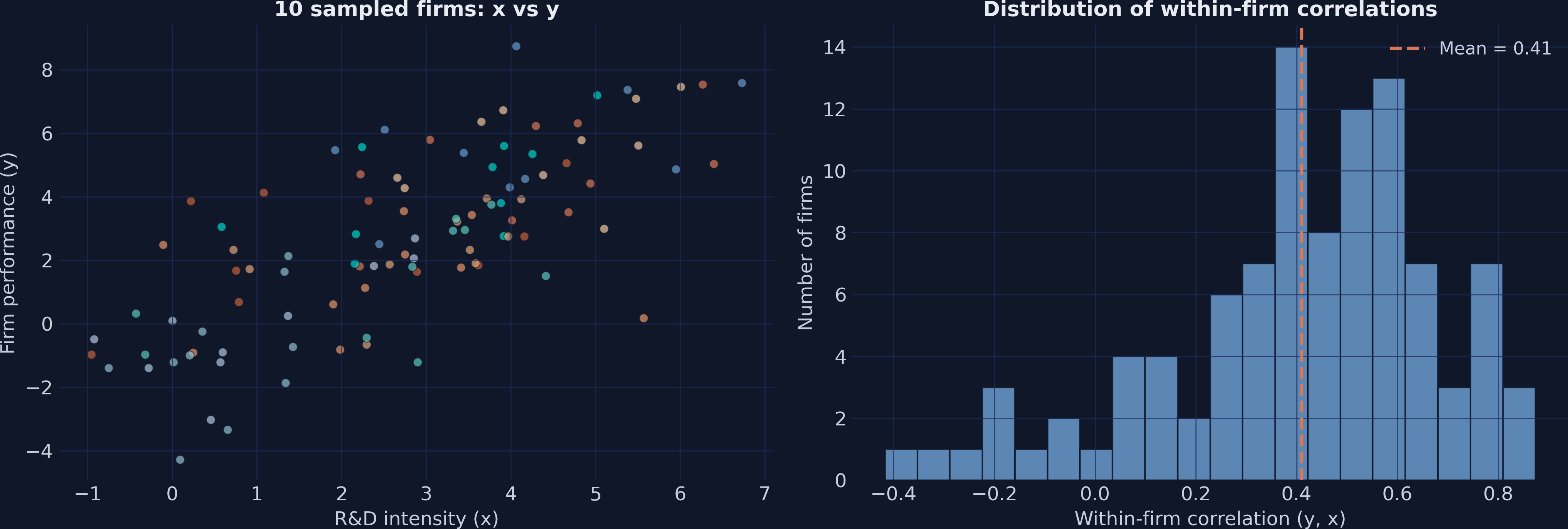
10 sampled firms cluster in distinct regions (left); within-firm \(y\)–\(x\) correlations center on 0.41 (right).

Left panel: each firm occupies a different region of x–y space — that’s between-firm variation, the confounded part fixed effects remove. Right: most firms show positive within-firm correlation around 0.41, less than 0.5 because AR(1) errors add noise. Between-firm std of y (2.46) exceeds within-firm std (1.67) — fixed effects will matter a lot.

Pooled OLS reports 1.03 — more than double the true 0.5

Model / SE	\(\hat\beta\)	SE	\(t\)
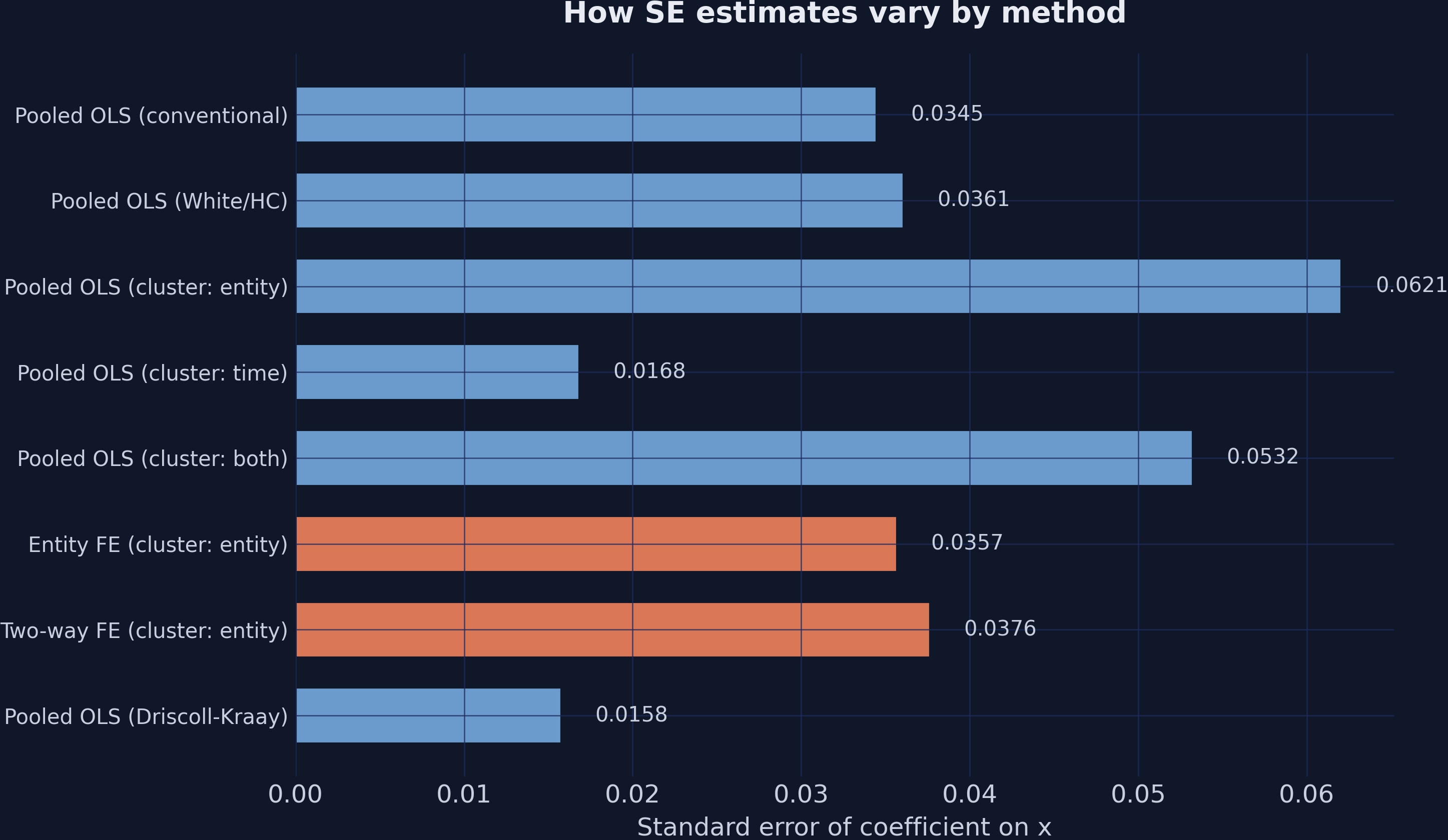
Pooled OLS (conventional)	1.0318	0.0345	29.9

The estimate is wrong, and the tiny SE makes us wrongly confident in the wrong number.

Omitted-variable bias in action: high-ability firms invest more in R&D and perform better, so the regression credits R&D for what ability does. The conventional SE of 0.0345 yields a t of 29.9 — doubly misleading: biased point estimate AND a too-small SE that ignores within-firm correlation. First lesson: a biased estimator with small SEs is worse than a noisy unbiased one.

White SEs barely move the needle — correlation, not heteroskedasticity, is the problem

\[\hat{\Sigma}_{\text{White}} = (X'X)^{-1}\left(\sum_{i=1}^{N} X_i'\,\hat{e}_i^{\,2}\,X_i\right)(X'X)^{-1}\]

White SE = 0.0361 vs conventional 0.0345 — the \(t\) slips only from 29.9 to 28.6.

The White estimator allows each observation its own variance, but still treats observations as independent. It cannot see that firm 1’s 2015 error correlates with its 2016 error. For panel data the binding problem is within-cluster correlation, so White helps almost nothing.

Clustering on firms inflates the SE by 80% — the honest correction

Model / SE	\(\hat\beta\)	SE	\(t\)
Conventional	1.0318	0.0345	29.9
White (HC)	1.0318	0.0361	28.6
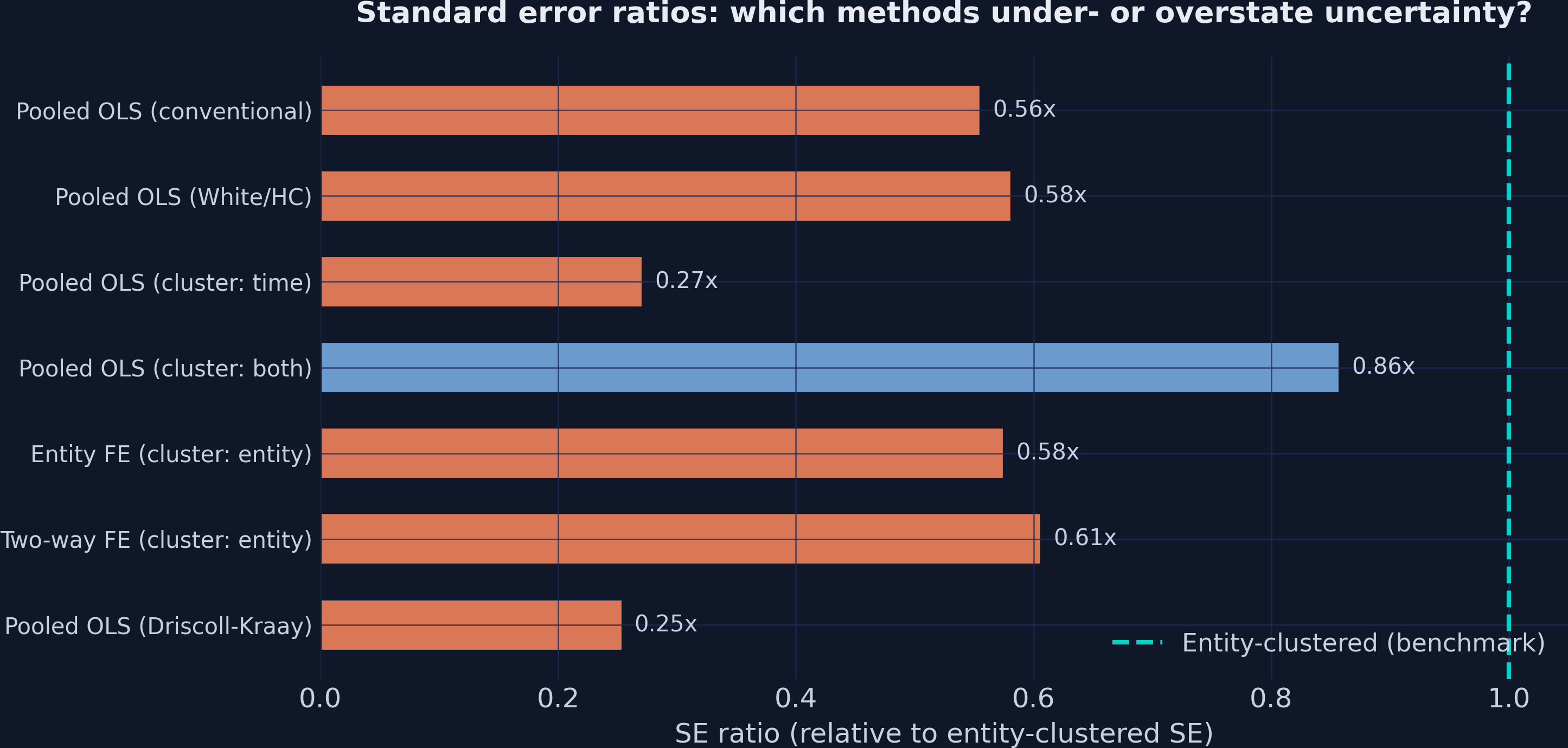
Cluster: entity	1.0318	0.0621	16.6

Ten observations from one firm carry far less than ten independent observations’ worth of information.

Entity clustering allows arbitrary correlation within a firm. The SE jumps to 0.0621 — 80% above conventional, nearly double White. The t falls from 29.9 to 16.6. Analogy: surveying 100 students across 10 classrooms gives you closer to 10 independent data points than 100. In a weaker-effect setting this correction could flip “significant” to “insignificant.”

Time clustering looks precise but lies: only 10 clusters break the asymptotics

Model / SE	\(\hat\beta\)	SE	\(t\)
Cluster: entity (100 groups)	1.0318	0.0621	16.6
Cluster: time (10 groups)	1.0318	0.0168	61.3
Cluster: both	1.0318	0.0532	19.4

Cluster on the dimension with \(\ge 40\)–\(50\) groups. Here that is firms (100), not years (10).

Time-clustered SEs are SMALLER than conventional, and t leaps to 61 — a trap. Clustered SEs rely on large-cluster asymptotics; 10 year-clusters is far too few. Two-way clustering (0.0532) sits between entity-only and time-only because the weak time dimension drags it down.

Fixed effects subtract each firm’s average — and the bias vanishes

from linearmodels.panel import PanelOLS
mod_fe = PanelOLS.from_formula("y ~ 1 + x + EntityEffects",
                               data=df_panel)
res = mod_fe.fit(cov_type="clustered", cluster_entity=True)
print(res.params["x"])       # 0.4829  — recovers the true 0.5
print(res.std_errors["x"])   # 0.0357

EntityEffects demeans within each firm, so the time-invariant ability mu_i drops out — beta is now estimated from within-firm variation only. The cov_type=“clustered” with cluster_entity=True handles the remaining AR(1) within-firm correlation. The post-FE clustered SE (0.0357) is actually smaller than the pooled clustered SE (0.0621) because FE removed the between-firm variation inflating residuals.

Fixed effects recover 0.48 — the bias was the model, not the SE

0.48

Entity FE \(\hat\beta\) (true \(\beta = 0.5\)); SE 0.0357 · pooled OLS gave 1.03

The single most important number transition: 1.03 (pooled, biased) to 0.48 (FE, ~unbiased). The residual gap of 0.017 is sampling noise, not systematic bias. No standard error correction could have done this — only changing the estimator. Adding TimeEffects barely moves it (0.4796), because the DGP’s time effects are weak.

One picture: no SE rescues a biased estimate; FE intervals cover the truth

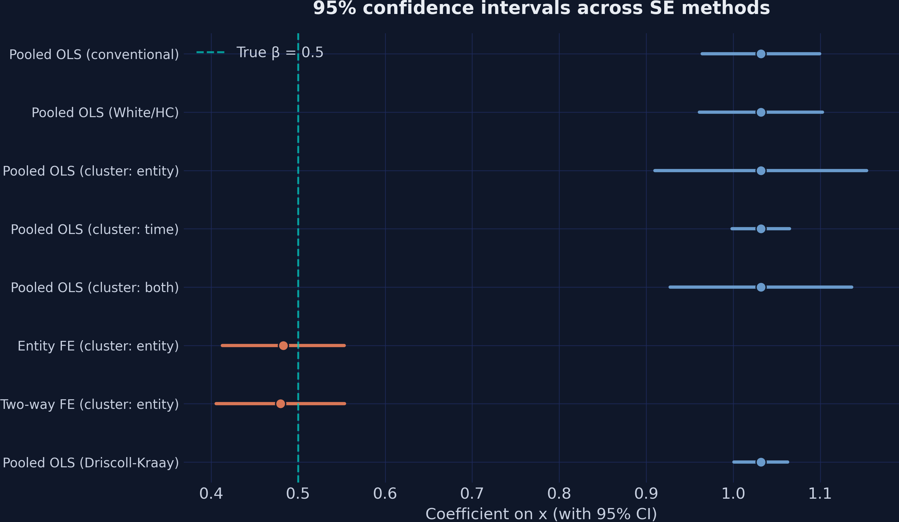
95% CIs across all eight methods. Teal dashed line = true \(\beta = 0.5\). Pooled intervals (right) miss it; FE intervals (orange) cover it.

The core visual message. All five pooled OLS intervals sit far to the right of 0.5 — none cover the truth, no matter the SE. The two FE intervals are centered near 0.5 and cover it easily. Standard errors set the WIDTH of the interval; the estimator sets its LOCATION.

Driscoll-Kraay targets cross-sectional shocks — weak here, vital elsewhere

Model / SE	\(\hat\beta\)	SE	\(t\)
Pooled (Driscoll-Kraay, BW=3)	1.0318	0.0158	65.4

Smallest SE in the deck — because firms are independent given their fixed effects in this DGP.

Driscoll-Kraay uses a Newey-West time kernel on cross-sectional averages — robust to spatial/cross-sectional dependence and serial correlation. Here cross-sectional dependence is weak, so DK is tiny. With strong common shocks (e.g. banks in a recession) and a long T, DK becomes the macro-panel standard. cov_type=“kernel”, kernel=“bartlett”, bandwidth=3.

The Resolution

Act III

Only Monte Carlo proves it: FE + entity-clustered rejects at 6.6%, near the nominal 5%

Rejection rates over 500 simulations, six FE+SE combinations. Dashed line = nominal 5%.

One CI plot could be lucky. The Monte Carlo runs 500 datasets from the same DGP and asks: how often does the 95% CI for the unbiased FE estimate miss the true 0.5? FE + entity-clustered rejects at 6.6% — close to 5% and within simulation noise. Conventional (6.0%) and White (6.4%) also do fine here because after FE the within-firm errors are nearly homoskedastic with 100 clusters to absorb the rest.

The too-small SEs sit at 0.55–0.58× the honest benchmark — understating uncertainty by ~40%

SE ratios relative to the entity-clustered benchmark. Ratios below 1.0 understate uncertainty.

The outlier from the Monte Carlo: FE + time-clustered rejects at 9.0%, nearly double 5% — 10 year-clusters violate large-cluster asymptotics, so the SEs are too small. This ratios figure normalizes everything to the entity-clustered SE: conventional and White on the pooled model sit at 0.55–0.58x, understating uncertainty by ~40%. TWFE + entity-clustered (3.2%) is mildly conservative — a benign property versus over-rejection.

Does fixing the SE make the estimate causal? No

Objection. “Clustered/robust SEs and a 6.6% rejection rate mean my coefficient is now the true causal effect.”

Response. Standard errors fix inference, never identification. The 0.48 estimate is unbiased here only because fixed effects removed the time-invariant confounder \(\mu_i\). A time-varying confounder would still bias \(\beta\) — and no SE could detect it.

Steelman, don’t strawman. Two distinct jobs: FE (and identifying assumptions) fix bias/identification; SEs fix the width of the interval. The Monte Carlo only validates that the SE controls size GIVEN an unbiased estimator. Strict exogeneity of x conditional on the firm effect is still an assumption.

The decision rule: fix the model first, then cluster on the larger dimension

Fix the bias

• Add fixed effects if there is entity-level heterogeneity
• SEs address precision, never bias
• Pooled \(1.03 \to\) FE \(0.48\)

Fix the inference

• Cluster on the larger dimension (firms: 100, not years: 10)
• Two-way clustering = safe default when both have \(\ge 40\)–\(50\) groups
• Driscoll-Kraay for long macro panels

Petersen (2009)’s framework. Order matters: model before standard errors. The FE + entity-clustered combination is the reliable micro-panel default — it addresses bias via FE and inference via clustering. Two-way clustering adds insurance against cross-sectional correlation.

Standard errors set the width of your conclusion — fixed effects set whether it is the right one.

The single takeaway. Every SE estimator left the biased pooled point estimate at 1.03; only fixed effects moved it to 0.48. Then, among honest estimators, only entity-clustering controlled size at the nominal level. Fix the model, then choose the SE.