Who Else Was Treated?

Three synthetic controls, one policy, and the interval that was 33 times too narrow

−16.87packs per capita, leak modelled

−5.50Nevada, from a law it never passed

33×how much too narrow the interval was

Carlos Mendez

Nagoya University (GSID)

August 4, 2026

Two Assumptions

Act I

The most replicated result in causal inference rests on two untested assumptions

The point of opening this way is that everybody knows the Prop 99 result and almost nobody states these two assumptions out loud. Naming them as assumptions rather than as machinery is the whole setup.

California’s Proposition 99, 1988. A 25-cent cigarette tax. The canonical synthetic control study.

One. The donor weights must be non-negative and sum to one — the simplex.

Two. No donor state absorbed any part of the treatment — SUTVA.

Neither is a fact about the world. Both are modelling choices, and both are testable.

This deck relaxes both. The effect survives. The claim that the donor pool was clean does not.

Thirty-nine states, thirty-one years, and one line that leaves the pack

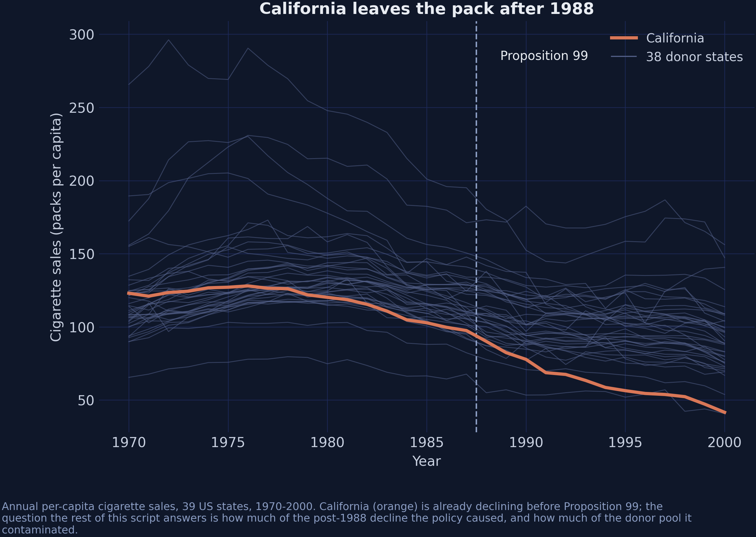
39 states · 1,209 rows · 18 pre-treatment years · 38 donors

California is already falling faster than the pack before the dashed line. That is why difference-in-differences fails here and why synthetic control exists at all.

Nevada is California’s only neighbour inside the donor pool

The exclusion list is doing quiet work here. Oregon and Arizona border California, but Abadie, Diamond and Hainmueller dropped both for having run their own tobacco-control programmes, which leaves Nevada as the only contiguous donor. Eleven states are absent from the panel for similar reasons. That is a gift and a limitation at once: the parameter is easy to interpret, and a single channel is thin evidence for a scalar.

Oregon and Arizona border California too.

Both ran their own tobacco programmes, so neither is a donor.

Eleven states are excluded altogether: AK, AZ, FL, HI, MD, MA, MI, NJ, NY, OR, WA.

The result: exactly one leak channel, and we can name it.

spatial_w has one non-zero entry. That is the whole spatial story, and it is why \(\rho\) is hard to pin down.

The simplex and SUTVA, written down

Read the first line as a sentence: find the mix of donor states whose weighted average tracks California over 1970 to 1987, subject to the mix being a genuine average — no negative weights, and the weights adding to one. The set delta is the simplex, and everything that distinguishes the three stages of this talk is a statement about delta. The second line is SUTVA. It throws away every argument of the potential outcome but one, which is why a classical synthetic control cannot report a spillover, cannot test for one, and cannot be wrong about one in a way you would notice.

\[\widehat{\alpha} = \arg\min_{\alpha \in \Delta} \sum_{t \le T_0}\Big(Y_{1t} - \alpha^{\top}\mathbf{Y}^{c}_{t}\Big)^2, \qquad \Delta = \Big\{\alpha : \alpha_j \ge 0,\ \textstyle\sum_j \alpha_j = 1\Big\}\]

\[\text{SUTVA:} \qquad Y_{jt}(\mathbf{D}) = Y_{jt}(D_j) \quad \text{for every donor } j\]

Relax the first and the donor pool changes. Relax the second and the counterfactual changes.

Python can now do all three stages without leaving one language

mlsynth’s PyPI release lags main at the same version string, which is why it gets a commit pin rather than a version pin.

pip install "scspill[numba]==0.2.1"
pip install "mlsynth[bayes] @ git+https://github.com/jgreathouse9/mlsynth.git@15f168bb"

mlsynth — 46 synthetic-control estimators behind one config dictionary.

scspill — the Bayesian spatial spillover model of Sakaguchi & Tagawa (2026), which returns two estimands.

Both are young. Both are pinned — one to a release, one to a commit.

Three relaxations, then two post-mortems

The three stages are nested: each keeps everything the previous stage assumed except one restriction, which it replaces with something weaker. That is what makes the comparison at the end meaningful — when the number moves, we know exactly which assumption moved it. The last two items are not relaxations but audits: why the R edition of this same analysis reports an interval 33 times narrower, and what an effective sample size of 3 actually means.

• Stage 1 — the simplex, as Abadie wrote it
• Stage 2 — the simplex replaced by a prior
• Stage 3 — SUTVA dropped, and a second estimand appears
• Reconcile and diagnose — why the R edition reports a very different interval, and what an effective sample size of 3 means

Three Stages on One Panel

Act II

Each stage drops exactly one restriction from the stage before

Stress that this is one regression, not three models. Stage 1 constrains alpha to the simplex. Stage 2 replaces that hard constraint with a prior — same alpha, weaker claim. Stage 3 keeps the prior and instead drops the assumption that the donors are clean. So when a number moves between stages, we know exactly which restriction moved it. That is the whole design of the talk.

Stage 1 — hard constraint: \(\qquad \alpha \in \Delta\)

Stage 2 — soft prior: \(\qquad \alpha_j \mid \lambda_j \sim \mathcal{N}(0, \lambda_j^2), \quad \lambda_j \mid \tau \sim \mathcal{C}^{+}(0,\tau)\)

Stage 3 — same \(\alpha\), but the donors are no longer clean:

\[\mathbf{Y}^{c}_{t} = \rho\big(\mathbf{w}\,Y_{1t} + W\mathbf{Y}^{c}_{t}\big) + X_t\beta + \mathbf{u}_t\]

One regression, not three models. When a number moves, we know which restriction moved it.

Stage 1 — the simplex picks five donors and stops

Note Nevada is already in the blend, carrying a quarter of the counterfactual — the one state we have reason to suspect. Section 4.1 of the post showed that sparsity can come from the data: a donor that is useless gets zero weight without any constraint forbidding it. Here it can equally have come from the constraint, and from the outside the two look identical. That is the question Stage 2 exists to ask.

common = dict(df=df, outcome="cigsale", treat="treated",
              unitid="state", time="year", display_graphs=False)

sc = mlsynth.VanillaSC(dict(common)).fit()

ATT (effect on California)	−18.43
pre-treatment RMSE	1.60
active donors	5 of 38
top-4 share of weight	98.6%

Utah 0.343 · Montana 0.254 · Nevada 0.242 · Connecticut 0.146 — and exactly zero for the other 33.

Is that sparsity in the data, or sparsity in the constraint? From the outside they look identical.

California and its synthetic are indistinguishable until 1988

The two series track closely until 1988 and separate steadily after it, reaching minus 26.7 packs by 2000. The pre-treatment gap is not exactly zero — it wanders between minus 3.5 and plus 5 packs, so an RMSE of 1.60 is an average over that wandering, not a promise that any single year fits well. Worth saying out loud: this reproduces the R edition’s minus 18.46 to within 0.04 packs, from a different package and a different optimiser, which is the strongest evidence either implementation gets that it is correctly coded.

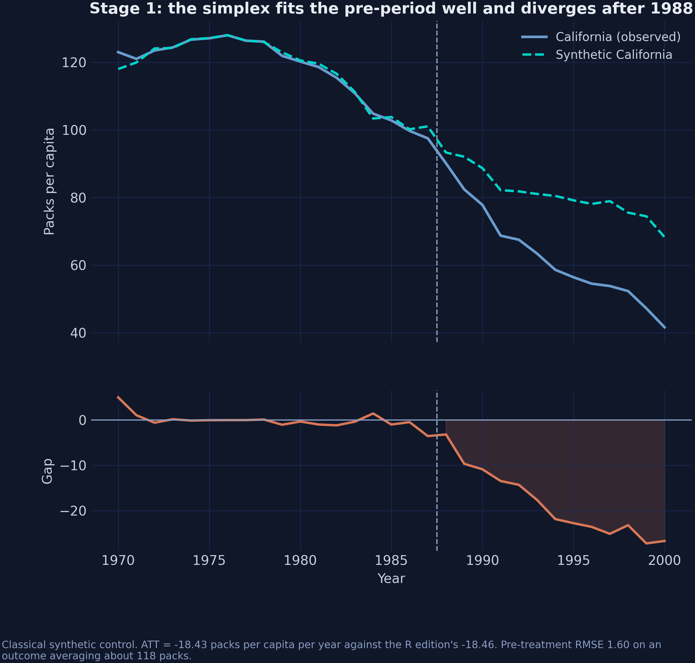
Zero gap before 1988; −26.7 packs by 2000.

The horseshoe makes zero the default without making it compulsory

Two properties that pull in opposite directions: enormous mass at zero, so a donor with nothing to contribute gets nothing; and tails heavy enough that a donor with a great deal to contribute is not shrunk into irrelevance. The name comes from the shrinkage factor kappa, one over one plus lambda squared, whose implied prior is a Beta one-half one-half — a U shape with peaks at 0 and 1. The Makalic–Schmidt step is the practical one: every half-Cauchy is a scale mixture of inverse gammas, so one auxiliary variable per scale gives closed-form conditionals throughout. Nothing is approximated.

\[\alpha_j \mid \lambda_j \sim \mathcal{N}\big(0, \lambda_j^2\big), \qquad \lambda_j \mid \tau \sim \mathcal{C}^{+}(0, \tau), \qquad \tau \sim \mathcal{C}^{+}(0, \sigma)\]

Infinite spike at zero. Cauchy tails. Most \(\lambda_j\) come out tiny; any single one can escape.

Sampling is closed-form via the Makalic–Schmidt inverse-gamma representation — an exact reparameterisation, not an approximation.

That is why both libraries run hundreds of thousands of iterations in seconds rather than hours.

Relax the simplex and the active donor pool multiplies by five

Point at the intervals before the points. Most of them straddle zero comfortably — the model is willing to entertain a role for these donors, but the data do not insist on one. The horseshoe did exactly what it promised: it made zero the default without making it compulsory. Two consequences of dropping the simplex are visible at once — the active count goes from 5 to 26, and the weights no longer sum to one. Neither is a defect.

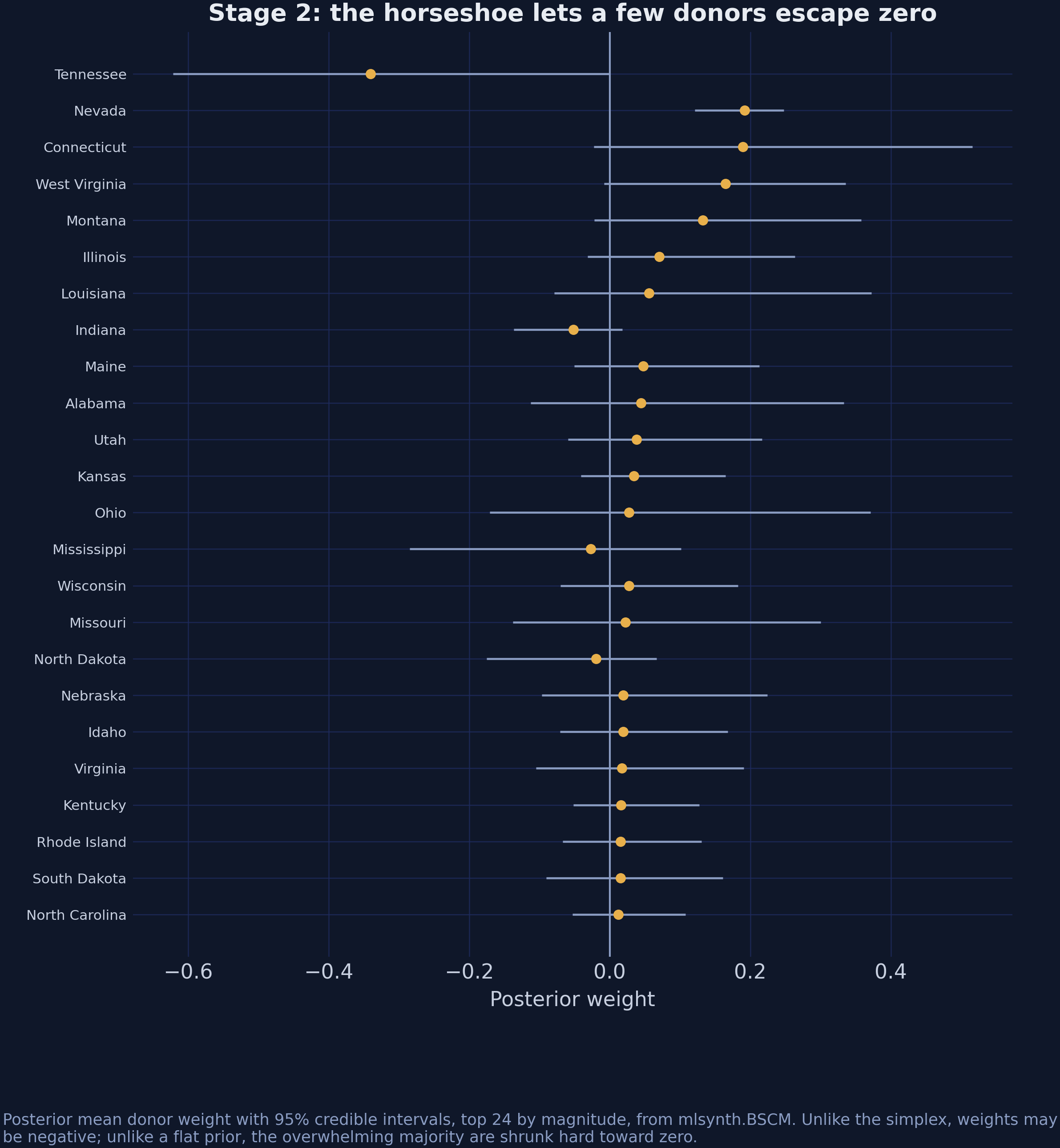
5 → 26 active donors. Almost every credible interval straddles zero.

Two Bayesian synthetic controls, one intercept apart

This is the slide people push back on. Both are horseshoe synthetic controls, and they land three packs apart. The reason is the intercept: BSCM fits beta-zero at 16.86 and its weights sum to 0.758, so its blend sits about 100 packs against California’s 118 and the intercept lifts it back. scspill has no intercept and standardises first. The tiebreaker is external — scspill’s rho-equals-zero case lands within 0.16 packs of the R edition, produced by entirely separate C++ code. Do not average them.

Estimator	ATT	Intercept	Weights sum
mlsynth.BSCM	−18.85	16.86	0.758
scspill at \(\rho = 0\)	−15.68	0	0.885
R edition, Stage 2	−15.84	0	—

\[\text{BSCM:}\ \ Y_{1t} = \beta_0 + \sum_j \alpha_j Y_{jt} + \varepsilon_t \qquad \text{scspill:}\ \ Y_{1t} = \sum_j \alpha_j Y_{jt} + \varepsilon_t\]

When two packages disagree about a model they both implement, check the equation before you check the sampler.

Drop SUTVA and the bias has a closed form

Derive it out loud in one line: add and subtract the weighted sum of the donors’ no-treatment outcomes. What a classical synthetic control reports is the true effect on California minus a weighted sum of the spillovers that landed on the donors — with the same weights used to build the counterfactual. Two consequences worth stating. If every spillover is zero the bias vanishes and classical synthetic control is right, so SUTVA is not a technicality but the whole justification. And the sign of the bias is the opposite of the sign of the weighted spillover, which is the fact the Nevada result turns on.

\[Y_{1t} - \sum_j \alpha_j Y_{jt} \;=\; \underbrace{\xi_{0t}}_{\text{what we want}} \;-\; \underbrace{\sum_j \alpha_j \xi^{c}_{jt}}_{\text{what we get for free}}\]

The bias is a product of two things: how much weight a donor carries, and how contaminated it is.

A filthy donor with zero weight is harmless. A slightly dirty one carrying half the counterfactual is not.

The simplex is gone; something took its place

Say plainly what has been traded. The simplex is gone, and something has taken its place: the assumption that some fixed alpha reproduces California’s untreated path exactly, in every pre-period. The weights may be negative and need not sum to one. It is not weaker in some absolute sense — it is untestable in a way the simplex is not, because the simplex’s price shows up as pre-treatment RMSE and this one does not show up anywhere.

\[\exists\, \alpha \in \mathbb{R}^{N} \;:\; Y_{1t}(\mathbf{0}) = \sum_j \alpha_j Y_{jt}(\mathbf{0}) \quad \forall t\]

Weaker than convexity, stronger than approximate fit — and untestable, because it leaves no RMSE behind.

The donors’ untreated path solves in closed form, and the nuisance block cancels

This is the technical heart of the talk. Substituting the treated unit’s equation into the donor system eliminates beta, the latent factors and the error variances — they all cancel. What is left depends only on alpha, rho, w, W and observed outcomes. That is why a weakly-mixing nuisance block does not poison the answer: there is nowhere for it to enter. It also localises the whole identification problem onto one scalar, which is what the rest of this talk is about.

With \(A = W + \mathbf{w}\alpha^{\top}\):

\[\mathbf{Y}^{c}_{t}(\mathbf{0}) = \big(I - \rho A\big)^{-1}\Big[\big(I - \rho W\big)\mathbf{Y}^{c}_{t} - \rho\,\mathbf{w}\,Y_{1t}\Big]\]

No \(\beta\). No factors. No error variances. They cancel.

The effects depend on \((\alpha, \rho, \mathbf{w}, W)\) and the observed data. Nothing else.

So the model’s weak identification has exactly one address: \(\rho\).

Weak identification you can locate is a manageable problem. Weak identification spread across a nuisance block is not.

One call runs both samplers and post-processes the spillovers

Everything spatial — w, W, the covariates — comes off the bundled panel, so there is nothing to align by hand. Half a million iterations for a 13-year effect looks excessive, and the post spends a whole section justifying it: the ATT is stable from about 100,000 draws onward, but the spatial parameter needs roughly five times that before its effective sample size reaches anything reportable. The rho-equals-zero comparator falls out of the same fit, which is why Stage 2 costs no extra MCMC at all.

result = SCSPILL({
    **panel.config_kwargs(),
    "m_iter": 500_000,
    "burn": 250_000,
    "seed": 20251022,
}).fit()

result.att                      # −16.87
result.effects_detail.att_scm   # −15.68, the ρ = 0 comparator, free
result.rho_hat                  # 0.316
result.spillover_panel          # 31 × 38: who else was treated

Stage 2 comes out of the Stage-3 fit at no extra cost. The model is nested.

The spatial parameter is clearly above zero

0.316

\(\widehat{\rho}\), 95% CrI [0.231, 0.403]. The interval excludes zero. The data reject \(\rho = 0\) — and with it, SUTVA on the donor pool.

The interval excludes zero, so the data reject the restriction that would collapse Stage 3 back to Stage 2. That is the SUTVA test, and it is a test the model nests rather than one bolted on afterwards. Resist reading precision into this number — the next slide is about exactly how much that interval is worth.

The two parameters leaning on one contiguity channel are the hard ones

Read the effective-sample-size column top to bottom. Sigma-squared has 204,000, the donor weights 10,000 to 26,000, rho has 137 and the price coefficient 388. Same chain. The point is not that the software is bad — it is that rho is the only parameter drawn by random-walk Metropolis rather than from a closed-form conditional, so its draws are heavily autocorrelated. Its posterior is actually tight: standard deviation 0.043 on a support 1.9 wide. Slow mixing is not the same thing as weak identification, and the distinction matters for what you tell a referee.

Parameter	Effective sample size (from 250,000 draws)
\(\sigma^2\)	204,095
\(\alpha\) (donor weights)	10,000 – 26,000
\(\beta\) (retail price)	388
\(\rho\)	137

\(\rho\) is the only parameter drawn by random-walk Metropolis rather than from a closed-form conditional, so consecutive draws are heavily correlated. The posterior itself is tight — SD 0.043 on a support 1.9 wide.

Slow mixing is not weak identification, and neither is a defect in the software.

Almost the entire spillover lands on one state

Walk the map first: on a linear colour scale almost every tile sits at the pale end, because one state absorbs an order of magnitude more than any other. The concentration is the finding, not a rendering artefact. Then the bars: Nevada at minus 5.50, then Idaho and Utah at about minus 0.49 — the two states that border Nevada, one ring further out — and everything beyond that second ring is two orders of magnitude smaller again. One limitation to state plainly rather than bury: scspill returns the effects panel as posterior means, so no donor-level spillover has a credible interval. “Noise” here means relative magnitude, not a tail probability. The interval evidence is on rho, not on Nevada. And slice from 1988 onward — the pre-treatment rows are fit residuals, not causal spillovers.

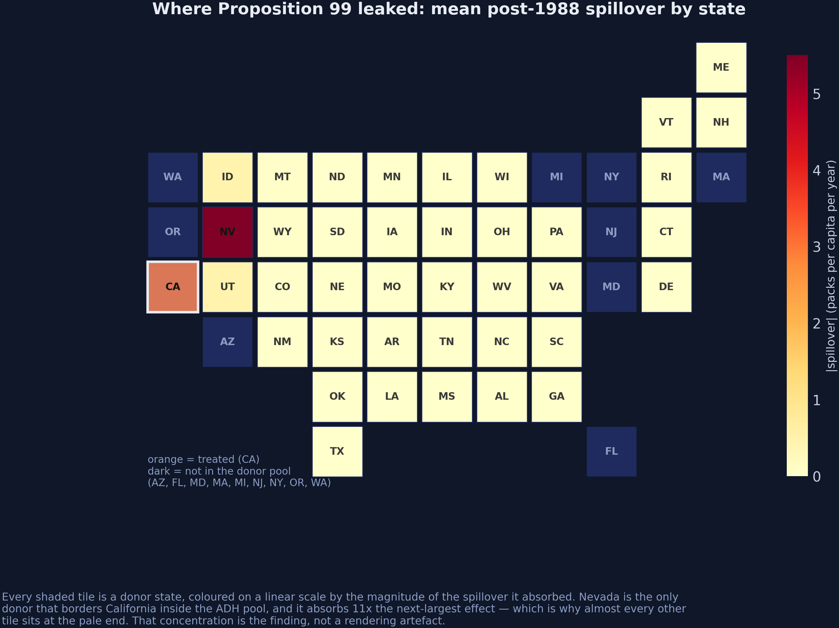
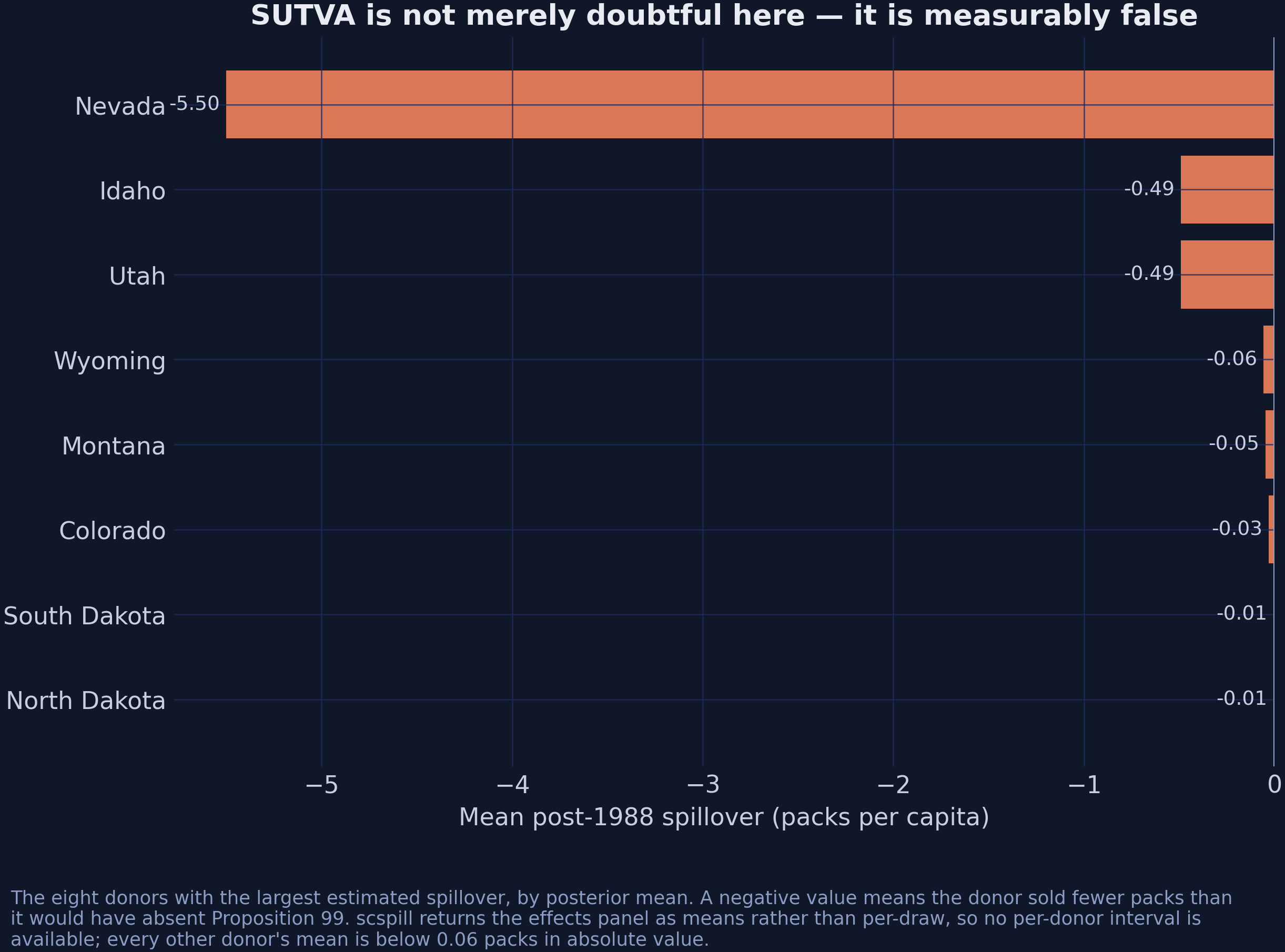
Nevada −5.50 · Idaho −0.49 · Utah −0.49 · every other donor under 0.06 packs.

The leak runs the opposite way to the obvious hypothesis

−5.50

Nevada’s sales came in below its no-treatment path. That looks like the campaign crossing the border, not the cigarettes — but the estimate cannot name the mechanism.

This is the sign surprise, and it is worth pausing on. The prior expectation was cross-border shopping raising Nevada’s sales; the estimate says they came in below their no-treatment path. Be careful not to over-claim: the post explicitly declines to name the dominant channel — advertising, media, social norms crossing a border that tax arbitrage also crosses — because nothing in the estimate identifies which. What it does say is that the net effect on Nevada ran the same way as the effect on California, not against it. Remember too that this number is a posterior mean with no interval around it.

Which means the classical estimate was biased toward zero

This inverts the intuition most audiences arrive with. The prior expectation is cross-border shopping raising Nevada’s sales, which would inflate the estimate. The estimate says Nevada’s sales fell. Negative spillover on a positively-weighted donor drags synthetic California down, so the classical comparison gives the policy less credit than it deserves. On the horseshoe weights that is 1.19 packs; on the simplex weights, where Nevada carries 0.242 instead of 0.200, it is 1.51. The classical estimate is the more contaminated of the two.

Donor	\(\alpha_j\)	\(\xi^{c}_j\)	\(\alpha_j \xi^{c}_j\)
Nevada	0.200	−5.50	−1.098
Utah	0.036	−0.49	−0.018
Idaho	0.012	−0.49	−0.006
Sum (all 38 donors)			−1.130

Purged minus contaminated: −1.186. The identity holds to 0.06 packs.

The residual is bookkeeping: the plug-in uses \(\widehat{\alpha}\); the purged ATT averages over paired draws.

Negative spillovers on positively-weighted donors push the estimate toward zero. Modelling the leak makes the effect larger.

The R edition’s interval is 33 times too narrow — and the R specification reproduces that exactly

The point estimates are close. The intervals are not remotely close, and “different language” does not explain a factor of 33. scspill documents six departures from the R replication code; three have escape hatches, so the Python can be put back into the R specification and run at the R edition’s own budget of 5,000 iterations. It reproduces rho to within 0.006 and the Nevada spillover to 0.03 packs — minus 3.750 against minus 3.778 — including an effective sample size of 3. That is not a coincidence to be explained away; it is the R sampler’s behaviour, faithfully reproduced. Which means the difference is a specification difference, not a porting error.

	ATT	95% CrI	Width
R edition (published)	−16.59	[−16.78, −16.39]	0.384
This post, corrected	−16.87	[−23.05, −10.33]	12.713

beta_prior="ridge"        # departure 2
propagate_alpha=False     # departure 3
adapt_rho=False           # departure 4

Back in the R specification: ATT −16.286 against −16.590, \(\widehat{\rho}\) 0.2282 against 0.2226, effective sample size 3.27 against 2.93.

Independent code, different language, reproducing the pathology — including an effective sample size of 3.

Chain length was never the problem — the interval was incomplete

Two separable failures, and the published interval failed both. Effective sample size asks: is the interval reliable — did the chain actually explore the posterior? At an ESS of 3, no. propagate_alpha asks a different question: is the interval complete — does it carry uncertainty about which states make up synthetic California? With alpha pinned at its posterior mean, no. Running the R specification a hundred times longer fixes the first and moves the width only from 0.48 to 0.70. The other factor of eighteen is the second. For the corrected run, adaptation lands acceptance at 0.444 against the 0.44 target and an effective sample size of 137.

Specification	Iterations	Width	ESS(\(\rho\))
scspill, R spec	5,000	0.482	3.3
scspill, R spec	500,000	0.702	66.9
scspill, corrected	500,000	12.713	136.8

A hundred times the iterations widens the interval by 45%. Propagating \(\alpha\) widens it by 1,700%.

Effective sample size asks whether the interval is reliable. propagate_alpha asks whether it is complete. The published interval failed both.

Report the effective sample size beside every credible interval, or the interval is decoration.

A memory layout was doing part of the modelling

Departure 1 is the most instructive kind of bug: the estimate simply answers a slightly different question than the one asked. Nothing crashes and nothing looks wrong. Departures 5 and 6 are different in kind — an omega-k conditional treating omega as a variance while its neighbours treated it as a precision, and an FFBS initialisation inconsistent with its own conditionals. Neither changes the California answer much, but both mean the R sampler was not converging to any posterior at all. It was converging to something, and that something had no interpretation.

Departure 1: the covariate array was indexed as \((N, T, K)\) when it was laid out as \((T, N, K)\).

Nothing crashes. Nothing looks wrong. Each state’s price is silently matched to another state’s sales.

It is also the one departure with no escape hatch worth using.

The only way out is to drop the covariates — one specification error for another.

Departures 5 and 6 were different: nobody spotted them. A Geweke joint-distribution test did.

The most dangerous bugs are the ones that return plausible numbers.

Artefacts shrink; errors do not

Explain the test before reading the figure. Draw parameters from the prior and simulate data from them: that is the marginal-conditional route to the joint distribution of parameters and data. Or simulate data once and then run one Gibbs sweep, repeatedly: that is the successive-conditional route. If every conditional in the sampler is correct the two routes target the same joint distribution, so any statistic’s mean must agree. The documentation’s rule for reading a failure is the one to quote: a genuine incoherence holds its position or grows as the chain lengthens, while a mixing artefact flips sign and shrinks. Here the maximum absolute z falls from 3.48 to 2.50, six of the eight statistics shrink, and the flag count goes from one to zero. A single Geweke run tells you almost nothing; two runs at different scales tell you which kind of failure you have.

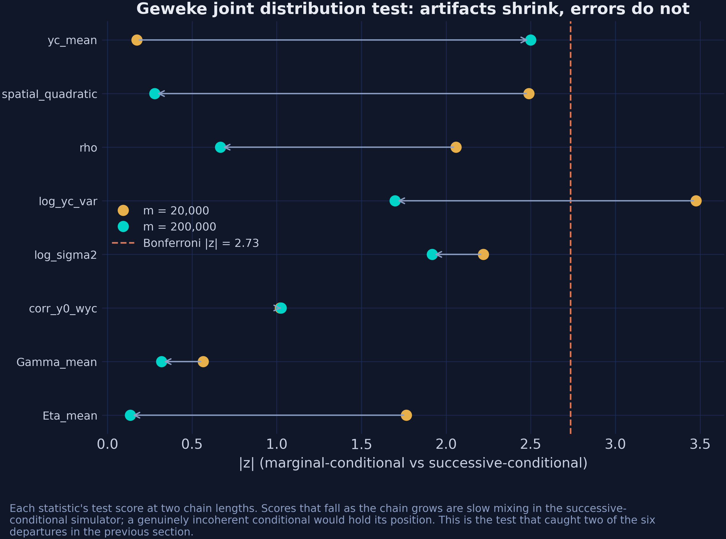
max \(|z|\) falls 3.48 → 2.50 and rejections go 1 → 0 as the chain grows tenfold. That is slow mixing, not an incoherent conditional.

The only prior that moves the answer is the one nobody calls a prior

Flag this before anyone reads the level off the axis. prior_sensitivity runs the simplified Step-2 kernel, not the production one, so the rho it reports here sits near 0.8 and must not be compared with the headline 0.316. What is comparable is the shape: the answer is flat across the inverse-gamma hyperparameters and across the step size, and moves only when the support itself is truncated to plus or minus 0.5. That is the finding — the support constraint is a prior too, and it is the one nobody reports.

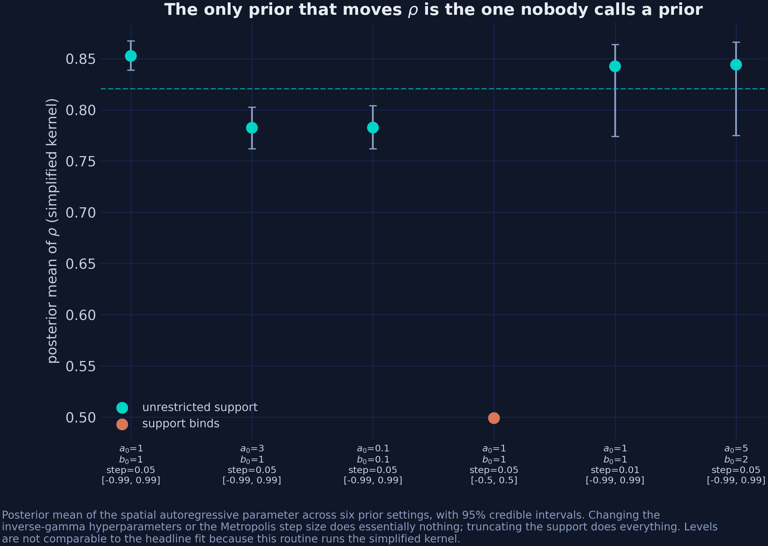
Sweeping \(a_0\), \(b_0\) and the step size moves \(\rho\) by 0.07. Truncating the support moves it by 0.32.

The strongest objection — and the answer

Deliver the objection as the strongest version of itself, then concede the part that is true. The SAR layer is a model of how outcomes co-move across a fixed, researcher-supplied graph, and swapping contiguity for a different graph would produce different spillovers. The post says exactly that in its discussion. The response is not that the assumption is harmless — it is that the alternative is rho equals zero, imposed silently and never reported. Making the assumption a parameter is what lets the data reject it. If pressed further, the honest concession is the identifying assumption itself: that some fixed unconstrained combination of donors reproduces California exactly. It is strong, and it is untestable.

Objection. The SAR layer does not make anything causal that was not causal before. You supplied the graph; a different graph gives different spillovers.

Response. Correct, and the post says so. But the alternative is not “no assumption” — it is \(\rho = 0\), imposed silently and never reported. Making the assumption a parameter is what lets the data reject it.

The choice is not between assuming and not assuming. It is between an assumption you can test and one you cannot.

What Survives Every Relaxation

Act III

Every stage of the ladder agrees on the sign and the scale

Read the ladder from the bottom up, then look at the hollow diamonds. Every stage lands between minus 15.7 and minus 18.8 packs — two libraries, four prior structures, one spatial layer and an independent third implementation — and the maximum disagreement with the R edition is 0.278 packs across four comparable stages. Do not over-claim beyond the figure: widening to the six comparable benchmark estimators in the post’s catalogue section stretches the range to minus 16.3 and minus 26.3, a wider band than this ladder shows, though still without changing the sign.

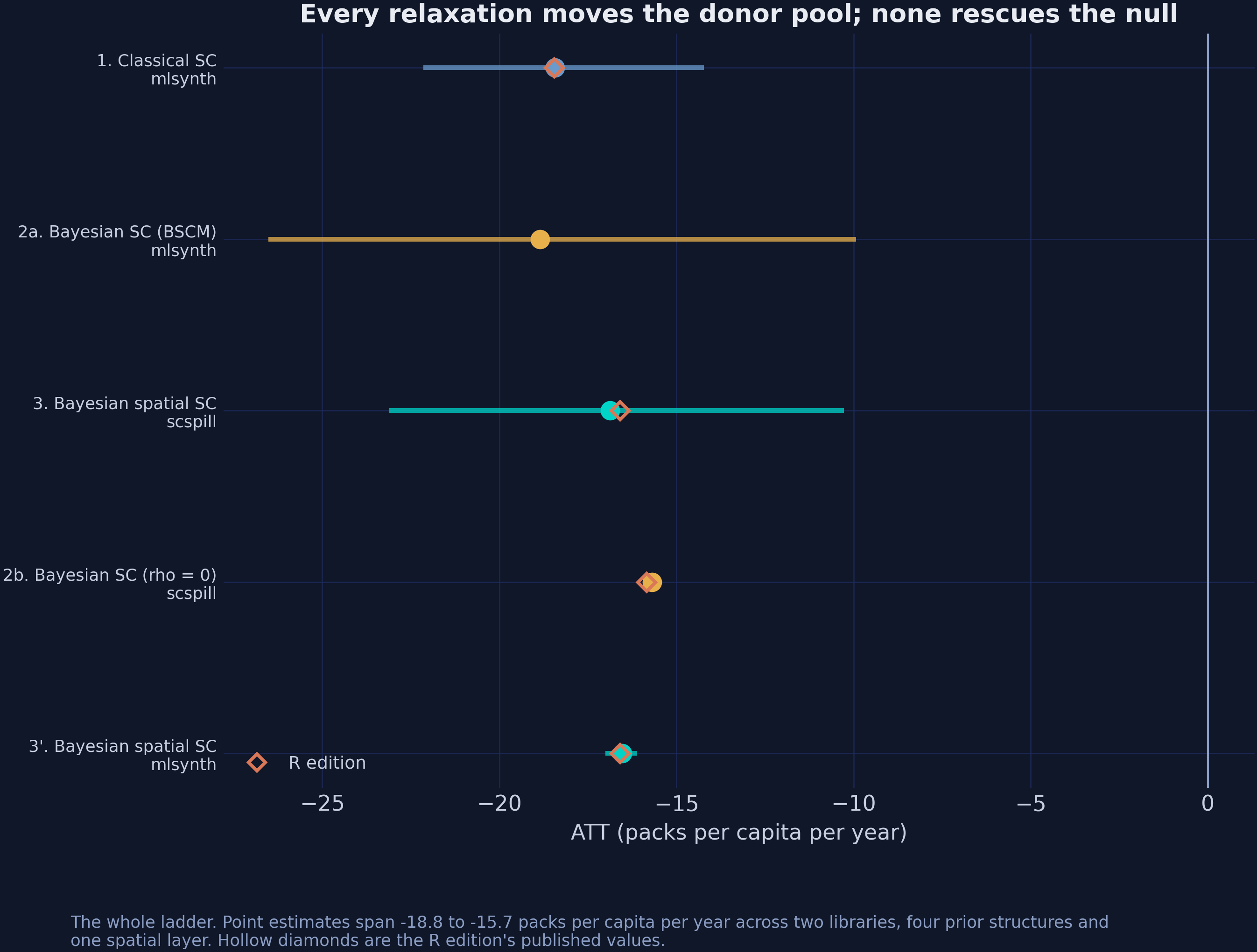
Two libraries, four prior structures, one spatial layer, one independent third implementation.

What Proposition 99 cost, and who else paid

−16.87

packs per capita per year for California — and −5.50 for a state that never voted on it

Two numbers, one policy. Minus 16.87 packs per capita per year for California once the leak is modelled, and minus 5.50 for Nevada, which never voted on it. The consequence for how the policy gets described: reporting only California’s number understates Proposition 99’s total public-health footprint, because a neighbouring state also smoked less.

Four things survive this deck

1. The effect is robust — −15.7 to −18.8 packs, every relaxation.
2. The donor pool is not — 5 donors or 26, depending on the constraint.
3. SUTVA is false here — 1.19 packs for California, 5.50 for Nevada.
4. The interval was the real error, not the point estimate.

Land these four and stop. The effect is robust and the classical estimate was fine for the headline number. The donor pool composition is not robust at all, and sentences of the form ‘synthetic California is mostly Utah and Nevada’ are closer to artefacts than findings. SUTVA is false here, but the correction is modest for California and large for Nevada — which is a different question, and the one classical synthetic control could not ask. On the simplex weights the California correction is 1.51 rather than 1.19, because the constraint pushed more weight onto the one leaking donor. And the interval, not the point estimate, was where the real error lived: two distinct failures, one diagnosable by effective sample size and one by asking what the interval is conditioning on.

Everything here is runnable today

Everything on this list ships with the post itself. The Colab notebook and the Quarto project reproduce every number in this deck; the web app lets you move rho by hand and watch the counterfactual respond; the data dictionary documents the panel and both spatial objects. Both packages are young, so both are pinned — one to a release, one to a commit — and the numbers are reproducible only under those pins.

• Full tutorial — carlos-mendez.org/post/python_sc_bayes_spatial
• R edition — carlos-mendez.org/post/r_sc_bayes_spatial
• Run it — Colab notebook, or the Quarto bundle with a hermetic .venv
• Web app — interactive \(\rho\) slider, donor comparator, trace diagnostics
• Data dictionary — the panel and both spatial objects

pip install "scspill[numba]==0.2.1"
pip install "mlsynth[bayes] @ git+https://github.com/jgreathouse9/mlsynth.git@15f168bb"

Let the data choose the donors, let the map say who else was treated, and let the ESS say whether the interval means anything.