The Augmented Synthetic Control Method: A Beginner's Tutorial with the Kansas Tax Cuts
1. Overview
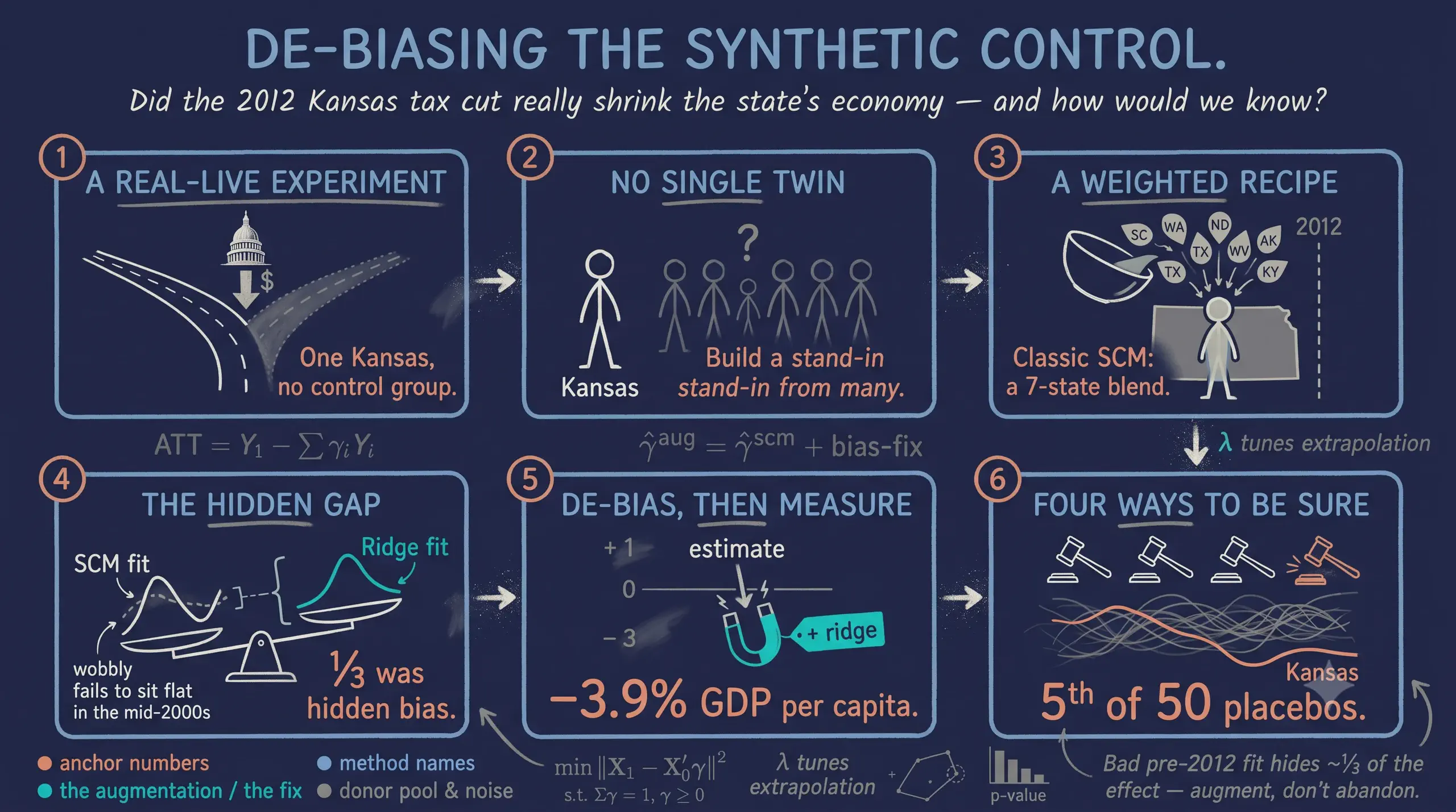
In May 2012, Kansas enacted one of the largest state tax cuts in recent U.S. history. Governor Sam Brownback called it “a real-live experiment” in supply-side economics: slash personal income taxes, and growth — the theory went — would follow. Did it? Answering that question is harder than it sounds, because we cannot rewind history and run Kansas without the tax cut to compare. There is only one Kansas, and it took the treatment.
The synthetic control method (SCM) offers a clever way out: if no single state is a good stand-in for Kansas, perhaps a weighted blend of several states can be. Build a “synthetic Kansas” from other states so that it matches the real Kansas before 2012, and its path after 2012 becomes the counterfactual — what Kansas’s economy would have done without the tax cut. The gap between the two is the estimated effect.
But classic SCM has an Achilles’ heel. It can only build the synthetic from a convex combination of donors — non-negative weights that sum to one — and sometimes no such combination matches the treated unit well enough. When the pre-treatment fit is imperfect, the estimate is biased, and the original authors of SCM recommend not using it at all. The Augmented Synthetic Control Method (ASCM) of Ben-Michael, Feller, and Rothstein (2021) rescues these cases: it keeps the interpretable SCM weights but adds an outcome model that estimates and subtracts the leftover bias.
This tutorial teaches ASCM for a single treated unit through the canonical Kansas example, using the augsynth R package. We deliberately move slowly: every method comes with the intuition first, then the equation, then the code, then the interpretation of real numbers. Inference in synthetic control is notoriously slippery, so we devote a full section to four different ways of asking “could this effect just be noise?”
If you want the multi-country, staggered-adoption version of these tools (
multisynth,augsynth_multiout), see the companion post Augmented Synthetic Control for Multiple Countries. This tutorial is the single-treated-unit foundation to read first.
1.1 Learning objectives
By the end of this tutorial, you will be able to:
- Implement classic SCM, Ridge ASCM, and covariate-augmented ASCM for one treated unit with
augsynth(). - Estimate the ATT of the 2012 Kansas tax cut on log GDP per capita, and read the pre-fit imbalance, the chosen penalty, and the estimated bias.
- Explain why the ridge bias-correction moves the estimate, and why it does so with almost no change to the donor weights.
- Assess statistical significance four ways — placebo/permutation, conformal, jackknife+, and the leave-one-donor jackknife — and explain when they disagree.
The roadmap below shows the path we will take. The branch point is the quality of the pre-treatment fit: when classic SCM matches Kansas well, augmentation changes little; when it cannot, ridge ASCM extrapolates just enough to de-bias the estimate.
flowchart TD
P["Kansas panel<br/>50 states, 1990-2016<br/>log GDP per capita"] --> Q{"Can donors match<br/>Kansas before 2012?"}
Q -->|"fit is good"| S["Classic SCM<br/>progfunc = None"]
Q -->|"fit imperfect<br/>(the mid-2000s gap)"| R["Ridge ASCM<br/>progfunc = Ridge"]
S --> W["SCM weights<br/>(convex recipe, 7 donors)"]
W --> B["+ Ridge outcome model<br/>estimate & subtract bias"]
R --> B
B --> Z{"Add covariates?"}
Z -->|"yes"| C["Covariate ASCM<br/>y ~ trt | Z"]
Z -->|"no"| A["ATT = actual - synthetic"]
C --> A
A --> I["Inference<br/>placebo · conformal · jackknife+ · jackknife"]
style P fill:#6a9bcc,stroke:#141413,color:#fff
style Q fill:#f5f5f5,stroke:#141413,color:#141413
style Z fill:#f5f5f5,stroke:#141413,color:#141413
style S fill:#d97757,stroke:#141413,color:#fff
style R fill:#d97757,stroke:#141413,color:#fff
style W fill:#6a9bcc,stroke:#141413,color:#fff
style B fill:#00d4c8,stroke:#141413,color:#141413
style C fill:#00d4c8,stroke:#141413,color:#fff
style A fill:#00d4c8,stroke:#141413,color:#fff
style I fill:#6a9bcc,stroke:#141413,color:#fff
2. Key concepts
Before the code, here are the seven ideas that carry the whole tutorial. Each card has a plain definition, a concrete example from the Kansas study, and an everyday analogy. The two hardest for newcomers are extrapolation (concept 3) and conformal inference (concept 7) — linger on those.
1. Synthetic control method (SCM). A weighted average of untreated “donor” units, built so its pre-treatment path matches the treated unit. The synthetic’s post-treatment trajectory is the estimated counterfactual; the gap to the real unit is the treatment effect.
Example
“Synthetic Kansas” is a blend of 7 states (South Carolina, Washington, Texas, …) chosen so that its pre-2012 GDP per capita tracks the real Kansas. After 2012, the gap is the effect of the tax cut.
Analogy
A stunt double assembled from several extras. Before the dangerous scene (treatment) the double mimics the star perfectly; during the scene it shows what would have happened to the star.
2. Donor pool. The set of untreated units the synthetic is built from. The treated unit is excluded, as is anyone else exposed to the treatment.
Example
The 49 U.S. states other than Kansas. None of them cut income taxes the way Kansas did in 2012, so each is a candidate ingredient for synthetic Kansas.
Analogy
The casting shortlist for the stunt double — only extras who did not perform the stunt are allowed to audition.
3. Convex hull and extrapolation. SCM weights are non-negative and sum to one, so the synthetic can only land inside the range spanned by the donors (it interpolates). Matching a treated unit that lies outside that range requires negative weights — extrapolation — which classic SCM forbids.
Example
In the mid-2000s, Kansas’s economy wobbles near the edge of what the donors can reproduce, so classic SCM leaves a stubborn gap there (a single quarter off by 0.043 log points). Ridge ASCM allows a controlled amount of extrapolation to close it.
Analogy
Mixing paint from stocked colours: you can blend them to get any shade between them, but you cannot use a negative amount of blue to get something brighter than your brightest blue.
4. Ridge penalty and bias correction. ASCM fits a ridge regression of donors’ outcomes on their lagged outcomes, predicts the residual imbalance, and subtracts it from the SCM estimate. A penalty λ controls how far the weights may leave the convex hull — large λ stays close to SCM, small λ extrapolates more.
Example
Augmentation moves the Kansas estimate from −0.029 to −0.040 and cuts the pre-fit imbalance from 0.083 to 0.062, reporting an estimated bias of 0.011 — about a third of the effect.
Analogy
A spell-checker for the counterfactual: SCM writes the first draft, and ridge fixes the systematic typos it can detect from the donors.
5. ATT — the estimand. The Average Treatment effect on the Treated: actual minus synthetic, in the post-treatment period, for the treated unit. It answers “what did the treatment do to Kansas,” not to an average state.
Example
The average post-2012 gap of about −0.04 log points ≈ a 3.9% shortfall in Kansas’s GDP per capita relative to its synthetic twin.
Analogy
The moment the stunt double keeps to the safe “no-stunt” script while the star veers off it — the distance between them is the effect of the stunt.
6. Pre-treatment fit (RMSPE / L2 imbalance).
How closely the synthetic tracks the treated unit before treatment. augsynth reports it as an L2 imbalance and as a percent improvement over naive uniform weights. A bad pre-fit makes any post-treatment gap meaningless.
Example
Classic SCM achieves L2 = 0.083 (79.5% better than uniform weights); Ridge ASCM tightens it to 0.062 (84.7%).
Analogy
How convincing the stunt double looks before the scene. If the audience can already tell them apart, nothing that happens during the scene is believable.
7. Conformal inference.
augsynth’s default test. Under the hypothesis of no effect, the post-treatment gaps should look like the pre-treatment gaps (just noise). Conformal inference checks whether the post-treatment residual “conforms” to the distribution of pre-treatment residuals, yielding a p-value and a pointwise confidence band.
Example
For classic SCM the 2012 Q3 effect is −0.041 with a 95% interval of [−0.070, −0.015] and p = 0.023 — the gap is larger than typical pre-period noise.
Analogy
A lie detector calibrated on a person’s resting readings. A post-event spike only counts as a signal if it exceeds their normal fluctuation.
3. Setup
The augsynth package is not on CRAN; install it once from GitHub. The other packages are standard. We fix a random seed because two of the inference procedures use resampling.
# install.packages("remotes")
# remotes::install_github("ebenmichael/augsynth")   # one-time install

library(augsynth)
library(dplyr)
library(tidyr)
library(ggplot2)
library(readr)

set.seed(20260608)

# Site colour palette used throughout
STEEL_BLUE  <- "#6a9bcc"   # synthetic control / SCM
WARM_ORANGE <- "#d97757"   # treated (Kansas) / actual
TEAL        <- "#00d4c8"   # ridge-augmented
A note on augsynth’s formula mini-language, which we will use repeatedly:
outcome ~ treatment— the minimal model: match on the entire pre-treatment outcome series.outcome ~ treatment | z1 + z2 + ...— also balance the auxiliary covariates listed after the|.progfunc = "None"— pure SCM, no outcome model.progfunc = "Ridge"— augment with ridge regression.scm = TRUE— use SCM (convex) weights as the starting point.
4. Data and key variables
The kansas dataset ships with augsynth. To keep this tutorial fully reproducible, we load it from a CSV in the post’s GitHub folder (a copy of the package’s kansas object), with a local fallback.
url    <- "https://raw.githubusercontent.com/cmg777/starter-academic-v501/master/content/post/r_augsynth/kansas.csv"
kansas <- if (file.exists("kansas.csv")) read_csv("kansas.csv") else read_csv(url)
kansas <- as.data.frame(kansas)

# The panel dimensions and the treated unit
length(unique(kansas$fips))          # number of states
range(kansas$year_qtr)               # time span
[1] 50
[1] 1990 2016
The panel is balanced: 50 U.S. states, observed every quarter from 1990 Q1 to 2016 Q1 — that is 105 quarters per state, 5,250 rows in all. The key variables are few and clear:
| Variable | Role | Meaning |
|---|---|---|
fips | unit id | State FIPS code (Kansas = 20) |
year_qtr | time | Year plus quarter, e.g. 2012.25 = Q2 2012 |
lngdpcapita | outcome | Natural log of gross state product per capita |
treated | treatment | 1 for Kansas from 2012 Q2 onward, 0 otherwise |
revstatecapita, revlocalcapita, avgwklywagecapita, estabscapita, emplvlcapita | covariates | Per-capita state revenue, local revenue, weekly wage, establishments, employment |
Let us look at exactly when treatment switches on:
kansas %>%
  filter(state == "Kansas" & year_qtr >= 2012 & year_qtr < 2013) %>%
  select(year, qtr, year_qtr, treated, gdp, lngdpcapita)
 year qtr year_qtr treated    gdp lngdpcapita
 2012   1  2012.00       0 143844    10.81687
 2012   2  2012.25       1 141518    10.79991
 2012   3  2012.50       1 138890    10.78051
 2012   4  2012.75       1 139603    10.78498
Interpretation. The treated flag is zero for Kansas through 2012 Q1 and one from 2012 Q2 (year_qtr = 2012.25) onward — exactly when the tax cut took effect. Notice the outcome already dips in the quarters right after: lngdpcapita falls from 10.817 to 10.781. But that raw dip is not yet a causal estimate — every state’s economy moved over this period. We need the counterfactual. With 89 pre-treatment quarters and 16 post-treatment quarters, we have a long history to pin down a credible synthetic Kansas — and, as we will see, a long pre-period is exactly what makes inference possible.
5. Exploratory view: why we need a synthetic control
ggplot() +
  geom_line(data = filter(kansas, fips != 20),
            aes(year_qtr, lngdpcapita, group = fips), colour = "grey78") +
  geom_line(data = filter(kansas, fips == 20),
            aes(year_qtr, lngdpcapita), colour = WARM_ORANGE, linewidth = 1.1) +
  geom_vline(xintercept = 2012.25, linetype = "dashed")
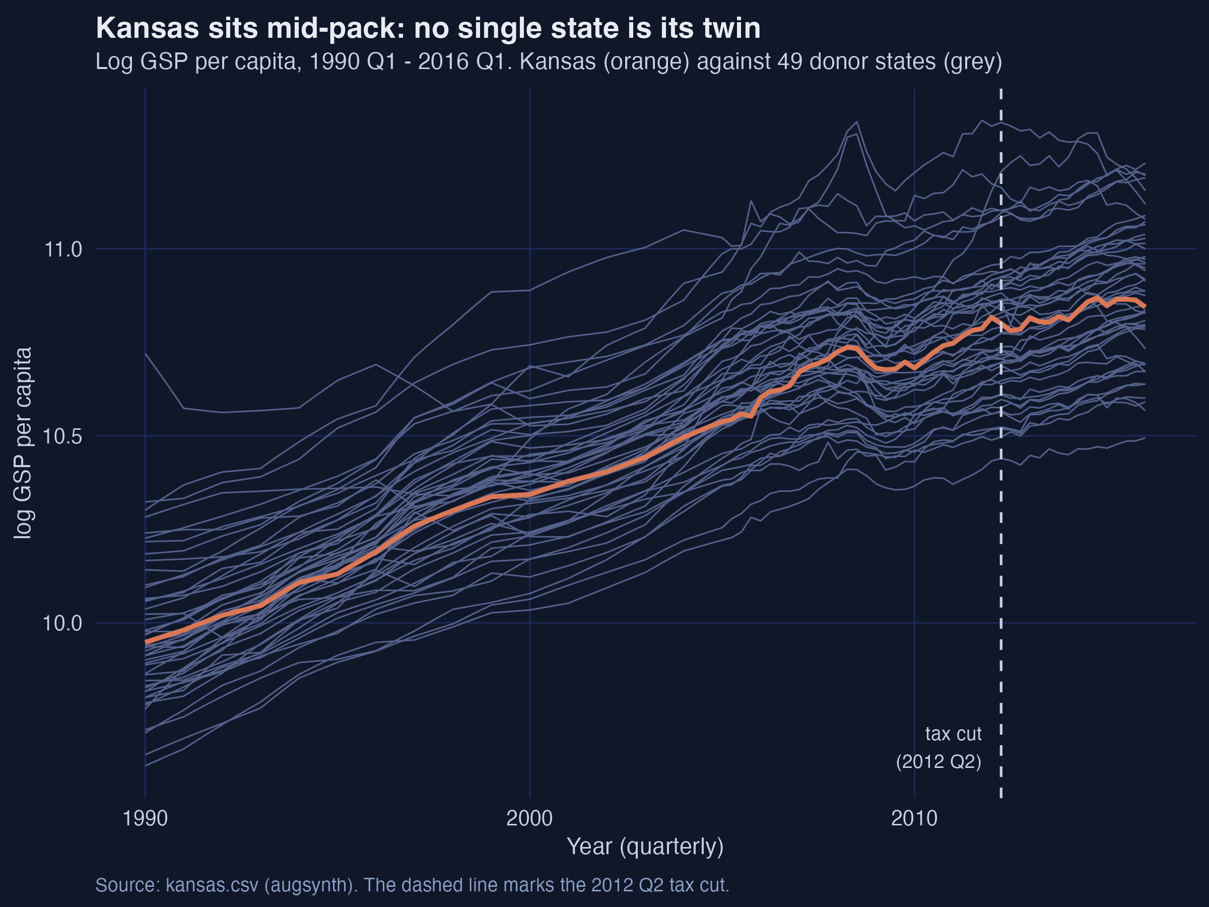
Interpretation. Kansas sits squarely in the middle of the pack and rises along with every other state for 26 years. This is the fundamental obstacle: there is no single state whose line lies on top of Kansas’s, so we cannot just pick “the most similar state” as a comparison. We have to construct a comparison by blending donors. The plot also previews the difficulty to come — in the mid-2000s the lines fan apart and Kansas wanders relative to its neighbours, which is precisely where a convex blend will struggle to keep up.
6. Baseline: the classic synthetic control
6.1 The idea, then the math
SCM picks donor weights so that the weighted donor outcomes reproduce the treated unit’s pre-treatment path as closely as possible, subject to two rules: the weights are non-negative and they sum to one. Those two rules are what keep the synthetic interpretable and prevent wild extrapolation.
Writing $X_1$ for Kansas’s vector of pre-treatment outcomes and $X_0$ for the matching matrix of donor outcomes, the SCM weights solve
$$\hat{\gamma}^{scm} = \arg\min_{\gamma} \| X_1 - X_0’ \gamma \|_2^2 \quad \text{subject to} \quad \sum_{i} \gamma_i = 1, \quad \gamma_i \ge 0$$
In words, this says: choose the weights $\gamma_i$ that make the blended donor history $X_0’\gamma$ as close as possible (in squared distance) to Kansas’s history $X_1$, while staying on the simplex (non-negative, summing to one). In code, $X_1$ is Kansas’s pre-2012 lngdpcapita and $X_0$ holds the 49 donors’ pre-2012 series; $\hat{\gamma}^{scm}$ becomes syn$weights.
Once we have the weights, the estimated effect in each post-treatment quarter $t$ is simply actual minus synthetic:
$$\hat{\tau}_t = Y_{1t} - \sum_{i} \hat{\gamma}_i^{scm}\, Y_{it}, \quad t > T_0$$
In words, the per-quarter ATT is Kansas’s realized outcome $Y_{1t}$ minus the weighted sum of donor outcomes (the synthetic). Here $T_0$ is the last pre-treatment period; in code $Y_{1t}$ is Kansas’s lngdpcapita and the weighted sum is predict(syn, att = FALSE).
6.2 Fitting it
syn <- augsynth(lngdpcapita ~ treated, fips, year_qtr, kansas,
                progfunc = "None", scm = TRUE)
summary(syn)
Fit to 50 units and 89+16 = 105 time points; 1 treated at year_qtr 2012.25.

7 donor units used with weights of 0.053 to 0.301
Average ATT Estimate (p Value for Joint Null):  -0.0294   ( 0.311 )
L2 Imbalance: 0.083
Percent improvement from uniform weights: 79.5%

Inference type: Conformal inference
Interpretation. Classic SCM builds synthetic Kansas from 7 donor states and estimates an average post-2012 ATT of −0.0294 log points. Because effects in logs are approximately percentages, that is a shortfall of about 2.9% in GDP per capita relative to the counterfactual. The pre-treatment L2 imbalance is 0.083, which augsynth tells us is 79.5% better than the naive alternative of weighting all 49 donors equally. The joint-null p-value of 0.311 is our first significance signal — and not a strong one — but hold that thought until the inference section.
We can see the synthetic control as a transparent recipe — the weights live in syn$weights, named by state FIPS code:
w <- syn$weights[, 1]
round(sort(w[w > 0.001], decreasing = TRUE), 3)   # the donors that actually matter
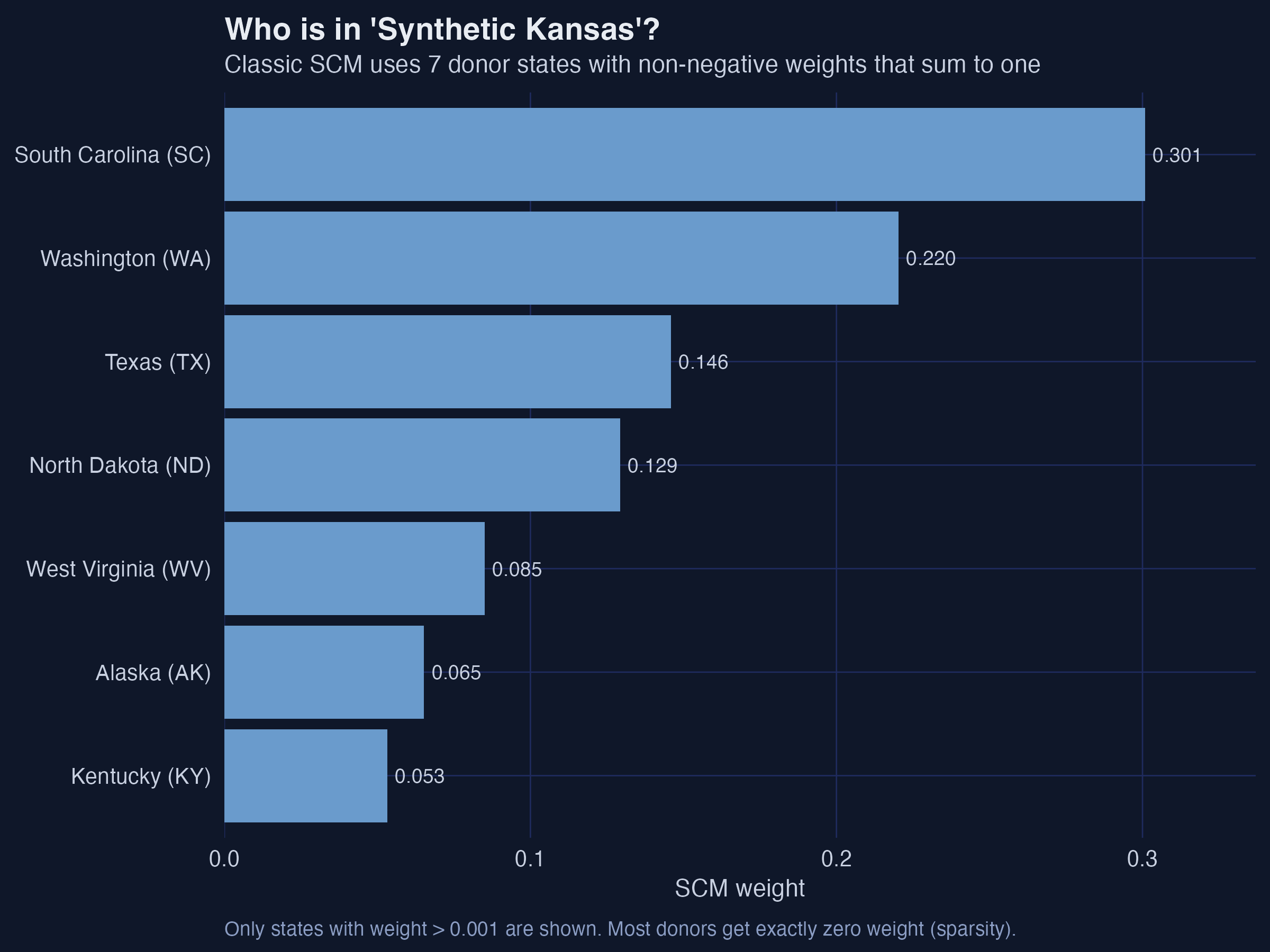
Interpretation. This is SCM’s signature virtue: 42 of the 49 donors get exactly zero weight, and the seven that remain form a recipe you can name and defend. South Carolina carries 30% of synthetic Kansas, Washington 22%, Texas 15%. The sparsity is not an accident — the simplex constraint pushes most weights to exactly zero. The cost of that interpretability is rigidity: if no convex recipe matches Kansas perfectly, SCM cannot do better, and the leftover mismatch becomes bias.
6.3 Seeing the counterfactual and the gap
plot(syn, plot_type = "outcomes") # actual Kansas vs its synthetic control
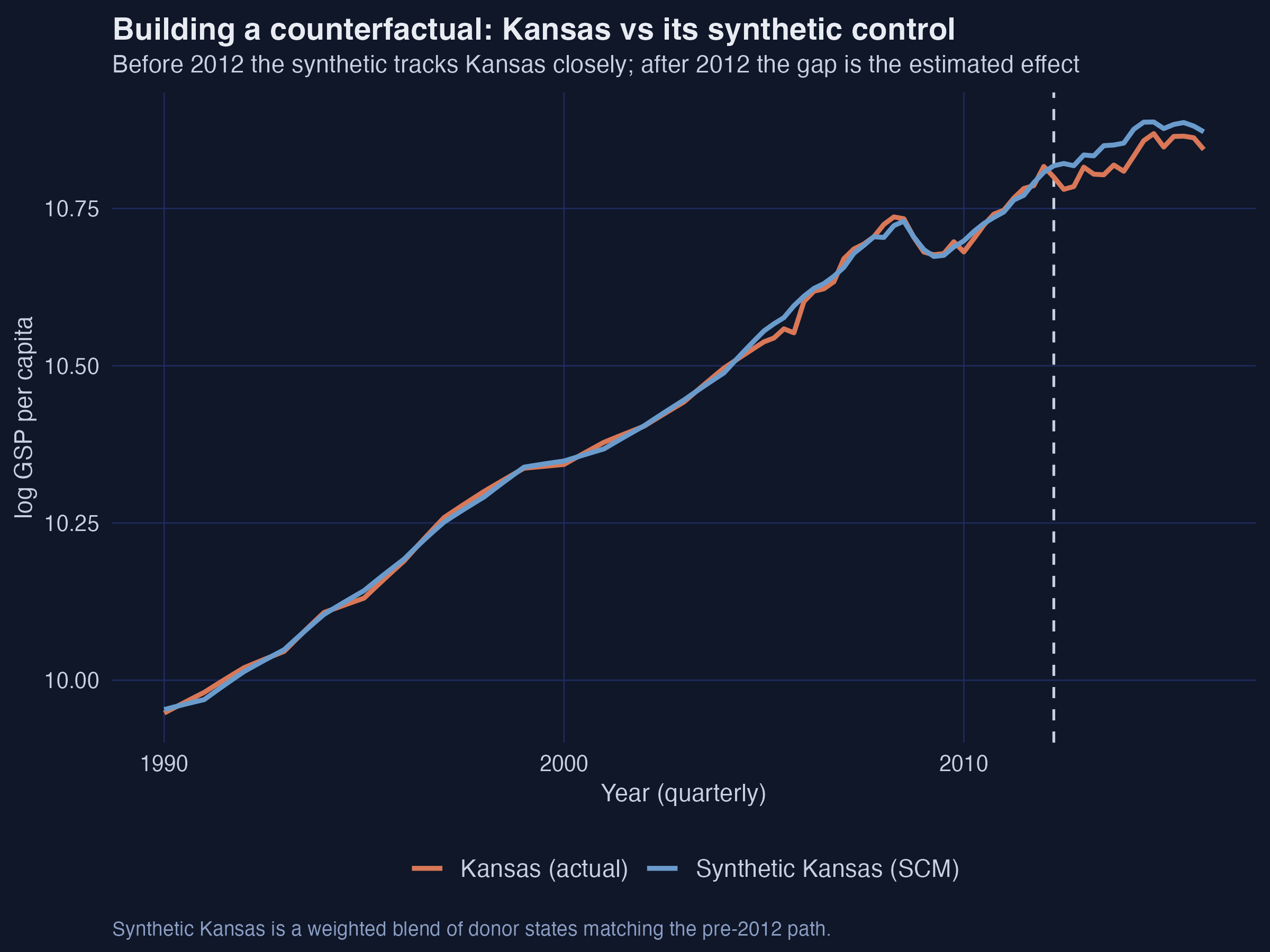
Interpretation. Before the dashed line the two series are nearly on top of each other — synthetic Kansas is a believable double. After 2012, the orange (actual) line slips below the blue (synthetic): Kansas grew more slowly than its counterfactual. That visible wedge is the treatment effect.
plot(syn) # the gap (actual - synthetic) with a pointwise conformal band
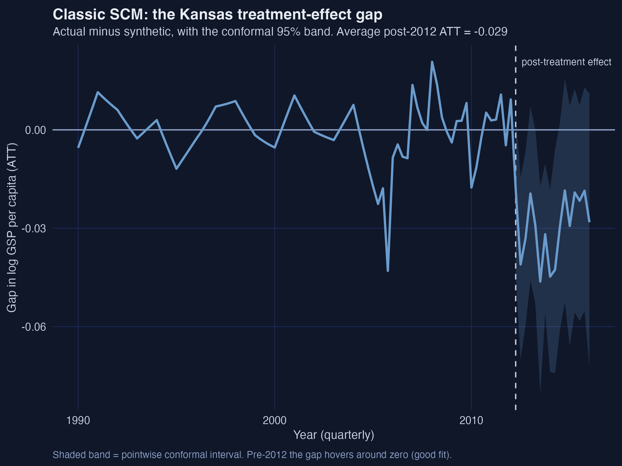
Interpretation. The gap plot isolates the effect on a single axis. Pre-2012 it oscillates around zero — but look at the dip near 2005–2006, which reaches −0.043 in one quarter. That is a pre-treatment gap, where the true effect is zero by definition, so it is pure imbalance: SCM simply could not match Kansas there. Post-2012 the gap turns reliably negative, deepest at 2013 Q3 (−0.046) and 2014 Q1 (−0.045). The shaded conformal band is wide, foreshadowing that significance will be a close call.
That stubborn mid-2000s imbalance is the motivation for everything that follows. It is exactly the situation Abadie and co-authors warn about — and exactly what ASCM was built to fix.
7. The augmentation: Ridge ASCM
7.1 The idea: estimate the bias, then subtract it
Here is the key insight. When the synthetic does not perfectly match Kansas before treatment, the post-treatment gap mixes two things: the real effect and the bias from that imperfect match. If we could estimate the bias, we could subtract it off. ASCM does exactly this by fitting an outcome model — a regression that predicts a unit’s outcome from its pre-treatment history — and using it to forecast how much the residual imbalance distorts the estimate.
The augmented counterfactual for the post-period can be written two equivalent ways. First, as “SCM plus a bias correction”:
$$\hat{Y}_{1T}^{aug}(0) = \sum_{i} \hat{\gamma}_i^{scm} Y_{iT} + \left( \hat{m}_{1T} - \sum_{i} \hat{\gamma}_i^{scm} \hat{m}_{iT} \right)$$
In words: start from the plain SCM counterfactual (the first term), then add a correction equal to the imbalance the outcome model $\hat{m}$ predicts (the parenthesis). If the model thinks Kansas’s history is systematically a little above what its donors’ weights reproduce, that term nudges the counterfactual accordingly. In augsynth this correction is reported as the “Avg Estimated Bias.”
The same estimator can be rearranged into a “model plus reweighted residuals” form, which is why ASCM is often described as doubly robust:
$$\hat{Y}_{1T}^{aug}(0) = \hat{m}_{1T} + \sum_{i} \hat{\gamma}_i^{scm} \left( Y_{iT} - \hat{m}_{iT} \right)$$
In words: predict Kansas directly from the outcome model ($\hat{m}_{1T}$), then correct it using the SCM-weighted residuals of the donors. If the SCM fit were already perfect, the residual term would balance out and ASCM would equal SCM — augmentation only does something when there is imbalance to fix.
The outcome model augsynth uses by default is ridge regression of donors’ outcomes on their lagged outcomes, with an L2 penalty:
$$\hat{\eta}^{ridge} = \arg\min_{\eta} \frac{1}{2}\sum_{i} \left( Y_i - X_i’ \eta \right)^2 + \lambda \| \eta \|_2^2$$
In words: fit a regression predicting the post-period outcome from the pre-period outcomes, but shrink the coefficients toward zero by an amount set by $\lambda$. The penalty $\lambda$ — in code, asyn$lambda — is the single dial that controls how aggressive the bias correction is.
7.2 Why ridge ASCM barely disturbs the weights
A beautiful result in the paper is that Ridge ASCM is equivalent to a penalized SCM: instead of forbidding negative weights outright, it lets the weights leave the simplex but penalizes how far they stray from the SCM solution:
$$\hat{\gamma}^{aug} = \arg\min_{\gamma} \frac{1}{2\lambda} \| X_1 - X_0’ \gamma \|_2^2 + \frac{1}{2} \| \gamma - \hat{\gamma}^{scm} \|_2^2 \quad \text{s.t.} \quad \sum_i \gamma_i = 1$$
In words: find weights that fit the pre-period well (first term) but stay close to the trustworthy SCM weights (second term). A large $\lambda$ makes the first term cheap, so the weights barely move from SCM; a small $\lambda$ lets them extrapolate more to chase a better fit. This is why, as we will see, the Kansas weights hardly change even as the fit improves.
And the improvement is guaranteed. The paper shows the augmented pre-treatment imbalance can only shrink relative to SCM:
$$\| X_1 - X_0’ \hat{\gamma}^{aug} \|_2 \le \frac{\lambda}{d^2 + \lambda} \, \| X_1 - X_0’ \hat{\gamma}^{scm} \|_2$$
In words: the augmented imbalance is the SCM imbalance multiplied by a factor that is always less than one. So augmentation never makes the pre-fit worse — it can only tighten it.
7.3 Choosing the penalty by cross-validation
How do we pick $\lambda$? augsynth uses leave-one-pre-period-out cross-validation: drop each pre-treatment quarter in turn, predict it, and measure the error. We then pick the $\lambda$ that the data say generalizes best.
asyn <- augsynth(lngdpcapita ~ treated, fips, year_qtr, kansas,
                 progfunc = "Ridge", scm = TRUE)   # lambda chosen by CV
plot(asyn, plot_type = "cv")
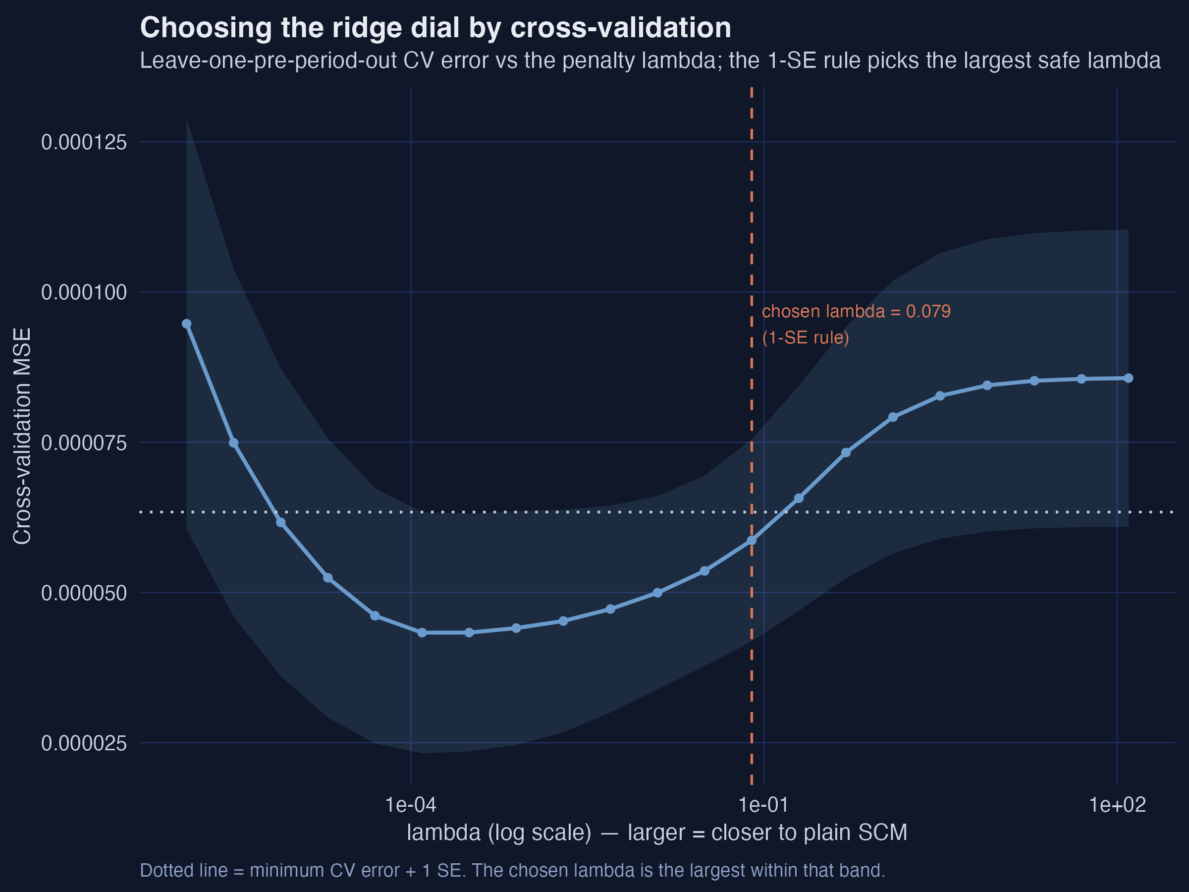
Interpretation. The CV curve is U-shaped: too small a $\lambda$ overfits the pre-period (right-hand rise is the opposite extreme, where the model becomes plain SCM), too large washes out the correction. By default augsynth applies the one-standard-error rule — it chooses the largest $\lambda$ whose error is within one SE of the minimum (here λ = 0.079). This is deliberately conservative: among statistically indistinguishable choices, it keeps the weights closest to the safe SCM solution. (Set min_1se = FALSE to instead minimize CV error and extrapolate more.)
7.4 What augmentation does to Kansas
summary(asyn)
49 donor units used with weights of 0.001 to 0.316
Average ATT Estimate (p Value for Joint Null):  -0.0401   ( 0.066 )
L2 Imbalance: 0.062
Percent improvement from uniform weights: 84.7%

Avg Estimated Bias: 0.011
Interpretation. Three numbers tell the story. First, the estimate deepens from −0.0294 to −0.0401 (about a 3.9% shortfall) — augmentation reveals a larger effect than plain SCM. Second, the pre-fit improves: L2 drops from 0.083 to 0.062 (84.7% better than uniform). Third, augsynth reports an estimated bias of 0.011 — its own measure of how much the SCM number was distorted by imperfect matching. That 0.011 is roughly one-third of the −0.040 effect, a striking confirmation of the paper’s warning that imperfect SCM fit can substantially understate the effect.
# both gap series come from predict(..., att = TRUE); see analysis.R for the full ggplot
scm_gap   <- predict(syn,  att = TRUE)
ridge_gap <- predict(asyn, att = TRUE)
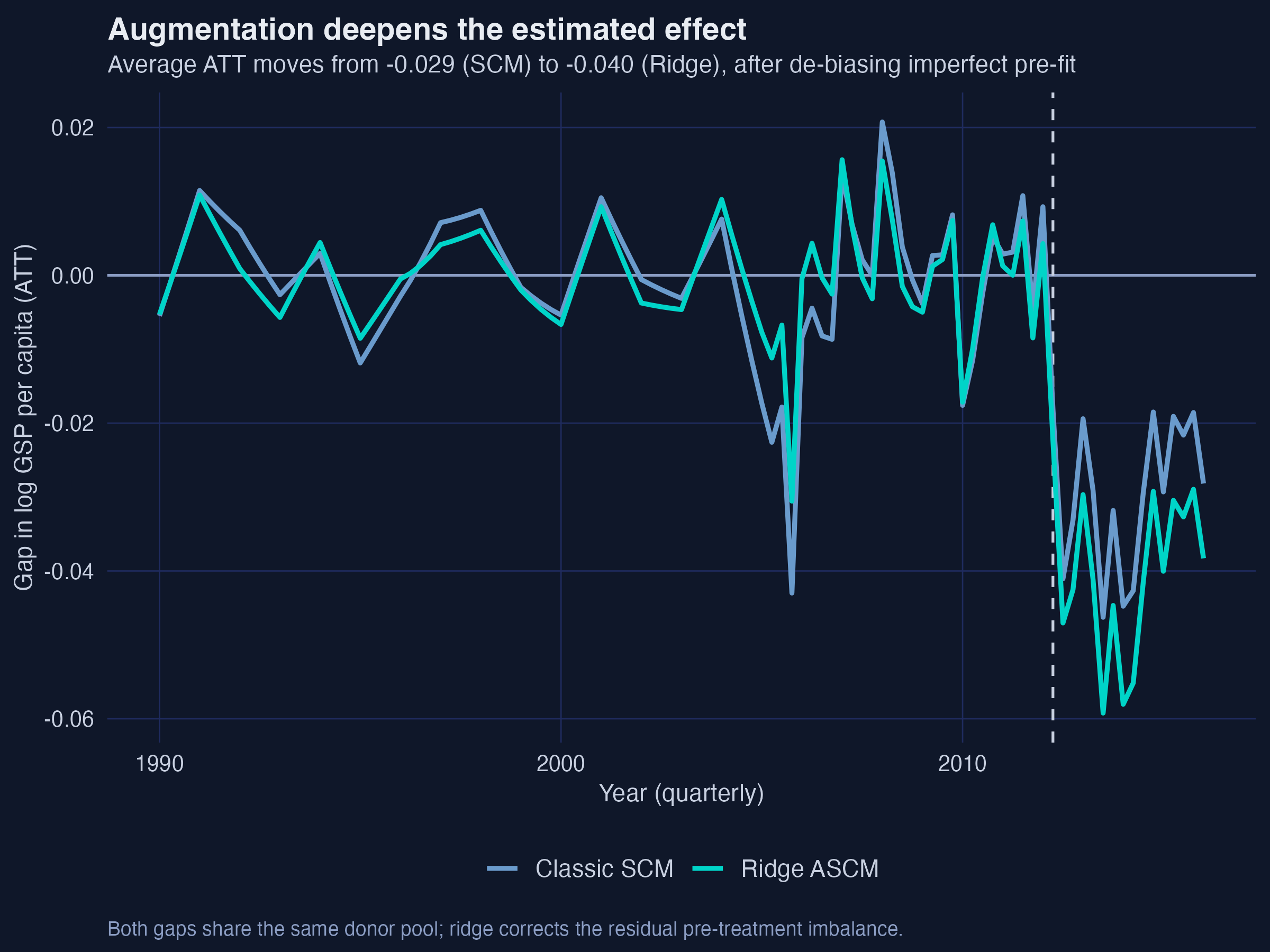
Interpretation. The two gaps share the same shape, but the teal ridge line dives a little deeper after 2012 — the visual signature of the bias correction. Crucially, this did not require throwing out the interpretable SCM recipe:
# How far did the weights actually move?
sqrt(mean((asyn$weights[,1] - syn$weights[,1])^2))
[1] 0.0147
Interpretation. The root-mean-square change in the donor weights is just 0.0147 — almost nothing. Although 21 donors now carry small negative weights (the controlled extrapolation), synthetic Kansas is essentially the same blend as before. Ridge ASCM bought a better fit and a de-biased estimate for the price of a tiny, principled departure from the convex hull. We can see where that price was paid:
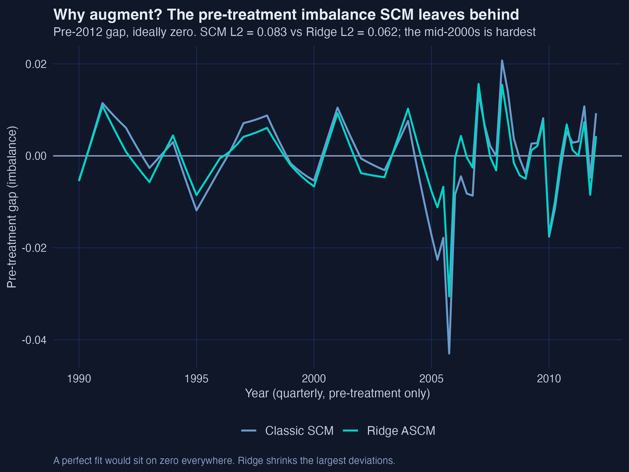
Interpretation. Restricting attention to the pre-period — where the gap should be zero — shows exactly what augmentation fixed. SCM’s worst quarter (2005 Q4, −0.043) is pulled back to −0.031 by ridge, and the rest of the turbulent mid-2000s is calmed too. That is the bias correction at work: it spent its small extrapolation budget precisely where classic SCM was failing.
8. Adding covariates
So far we matched only on the history of the outcome. But augsynth can also balance auxiliary covariates — state revenue, wages, establishments, employment — by listing them after a | in the formula. Both the lagged outcomes and the covariates then enter the SCM balancing problem and the ridge outcome model:
$$\min_{\eta_x, \eta_z} \frac{1}{2}\sum_{i} \left( Y_i - X_i’ \eta_x - Z_i’ \eta_z \right)^2 + \lambda_x \| \eta_x \|_2^2 + \lambda_z \| \eta_z \|_2^2$$
In words: the outcome model now uses both the lagged outcomes $X$ (with coefficients $\eta_x$) and the covariates $Z$ (with coefficients $\eta_z$), each with its own ridge penalty. The covariates give the synthetic more ways to resemble Kansas than the outcome path alone.
covsyn <- augsynth(lngdpcapita ~ treated | lngdpcapita + log(revstatecapita) +
                     log(revlocalcapita) + log(avgwklywagecapita) +
                     estabscapita + emplvlcapita,
                   fips, year_qtr, kansas, progfunc = "ridge", scm = TRUE)
summary(covsyn)
49 donor units used with weights of 0.004 to 0.356
Average ATT Estimate (p Value for Joint Null):  -0.0609   ( 0.124 )
L2 Imbalance: 0.054
Percent improvement from uniform weights: 86.6%

Covariate L2 Imbalance: 0.005
Percent improvement from uniform weights: 97.7%

Avg Estimated Bias: 0.027
Interpretation. Adding the six covariates sharpens balance on two fronts: the outcome imbalance falls to 0.054 and the covariate imbalance to 0.005 — a 97.7% improvement over uniform weights. With the additional structure, the estimate deepens again to −0.0609 (≈ −5.9%). The covariates fix dimensions of similarity that lagged outcomes alone miss — for instance, matching Kansas’s employment and wage levels, not just its GDP trajectory.
Two further options are worth knowing but not belaboring. Residualizing (residualize = TRUE) first regresses the outcome on the covariates and fits ASCM on the residuals; on Kansas it drives covariate imbalance to exactly zero and gives an ATT of −0.0548. The simplest possible outcome model, a unit fixed effect (fixedeff = TRUE, which de-means each series), gives −0.0335 — between plain SCM and ridge. Every route agrees on the sign and the rough size of the effect.
9. Inference: could this just be noise?
This is the part students find hardest, and for good reason: a synthetic-control estimate is a difference between two estimated curves, built from one treated unit. Classical standard-error formulas do not obviously apply. augsynth ships four tools, and they can give different verdicts. The shared question they all answer is: is the post-treatment gap bigger than what we would see by chance? They differ in how they define “by chance.”
We run all four on the Ridge ASCM fit (only the ridge estimator supports standard errors).
9.1 Placebo / permutation tests (the classic approach)
The original SCM inference, due to Abadie and co-authors, is a placebo test. The logic: if the tax cut truly moved Kansas, then re-running the whole analysis pretending some untreated donor was “treated” should usually produce a much smaller gap. Do this for every donor, and you get a distribution of placebo effects to compare Kansas against.
A common summary statistic is the RMSPE ratio — post-treatment fit error divided by pre-treatment fit error — which rewards units that tracked well before and diverged after. The permutation p-value is Kansas’s rank in that distribution:
$$p = \frac{\#\{\, i : r_i \ge r_1 \,\}}{N}, \qquad r_i = \frac{\text{RMSPE}_i^{\text{post}}}{\text{RMSPE}_i^{\text{pre}}}$$
In words: compute each unit’s post/pre error ratio $r_i$, then ask what fraction of all units (including Kansas, unit 1) have a ratio at least as large as Kansas’s. A small fraction means Kansas stands out.
plot(asyn, plot_type = "placebo") # switches to permutation inference
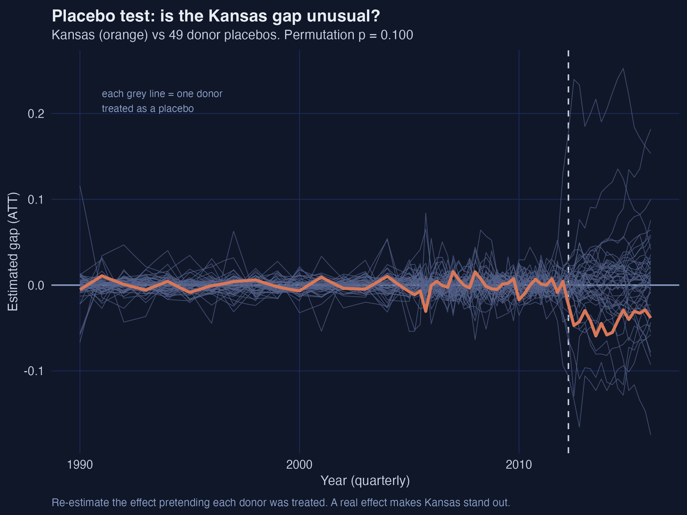
Interpretation. Kansas’s pre-2012 line is buried in the grey chorus — a good fit, so it belongs in the comparison. After 2012 it drops toward the bottom edge, but it is not the single most extreme path. Its post/pre RMSPE ratio of 6.36 ranks 5th of 50, giving a permutation p = 0.10. Read honestly: Kansas’s response is unusual, but a handful of placebo states show swings just as large, so the placebo test alone cannot rule out chance at the 5% level. The placebo test is intuitive and assumption-light, but it has low power with a small donor pool and assumes Kansas is exchangeable with the donors.
9.2 Conformal inference (the modern default)
augsynth’s default is conformal inference (Chernozhukov, Wüthrich, and Zhu, 2021). It tests a sharp null — “the effect equals $\tau_0$” — by checking whether, after subtracting $\tau_0$, the post-treatment residual looks like an ordinary draw from the pre-treatment residuals. Inverting the test over a grid of $\tau_0$ values yields a confidence interval. The p-value for “no effect” is
$$p(\tau_0) = \frac{1}{T_0 + 1} \left( 1 + \sum_{t=1}^{T_0} \mathbf{1}\{\, |\hat{u}_t| \ge |\hat{u}_{T}| \,\} \right)$$
where the residual at the candidate effect $\tau_0$ is
$$\hat{u}_t = Y_{1t} - \tau_0 \cdot \mathbf{1}\{t > T_0\} - \sum_{i} \hat{\gamma}_i(\tau_0)\, Y_{it}$$
In words: under the null, the post-treatment residual $|\hat{u}_T|$ should be no more extreme than a typical pre-treatment residual $|\hat{u}_t|$. The p-value is the share of pre-periods whose residual is at least as large — a long pre-period (89 quarters here) is what gives this test its resolution.
summary(asyn)$average_att # the conformal joint-null p-value
Average Post-Treatment Effect -0.0401 p = 0.066
Interpretation. The conformal joint-null p-value is 0.066 — borderline, just above the conventional 5% line. But the pointwise picture (the band in the gap plots) is sharper: several individual quarters clear significance, including 2013 Q3 (−0.059, p = 0.024) and 2014 Q1 (−0.058, p = 0.018). Conformal inference is the most robust of the four here because it does not require Kansas to be exchangeable with the donors and it exploits the long pre-period.
9.3 Jackknife+ over time
The jackknife+ builds a confidence interval for the average effect by leaving out one pre-treatment period at a time, refitting, and using the spread of the leave-one-out prediction errors to bound the estimate.
summary(asyn, inf_type = "jackknife+")$average_att
Average Post-Treatment Effect -0.0401 95% CI [-0.0576, -0.0206]
Interpretation. The jackknife+ interval [−0.058, −0.021] excludes zero — by this criterion the average effect is significant. It is the only one of the four that gives a clean “significant” verdict for the average, because it asks a different question: how stable is the estimate when we perturb the time dimension, rather than whether Kansas is special among states.
9.4 Leave-one-donor jackknife
The final tool drops one donor at a time, recomputes the ATT, and forms a standard error from how much the estimate moves — the classic “how sensitive is this to any single comparison unit?” check.
summary(asyn, inf_type = "jackknife")$average_att
Average Post-Treatment Effect -0.0401 Std.Error 0.0242
Interpretation. With a standard error of 0.0242, the Wald interval is −0.040 ± 1.96 × 0.024 = [−0.088, 0.007], which includes zero. The reason is intuitive: synthetic Kansas leans heavily on a few donors (South Carolina alone is 30%), so dropping one of them can move the estimate appreciably, inflating the standard error. This is the most conservative of the four.
9.5 Putting the four together
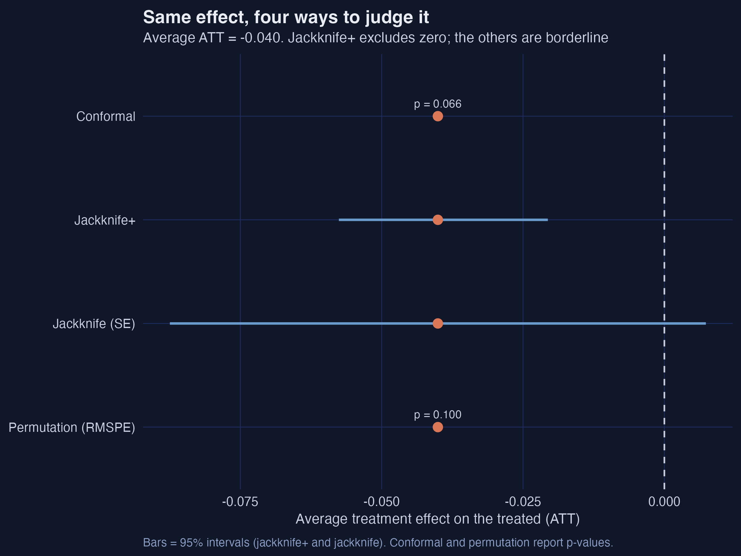
Interpretation. This single figure is the lesson of the section. The point estimate is the same −0.040 in all four; what differs is the uncertainty. The methods disagree because they probe different sources of variation — over time (conformal, jackknife+) versus over units (permutation, leave-one-donor jackknife) — and make different exchangeability assumptions. The honest conclusion is not “significant” or “not significant” but a nuanced one: a real, modest negative effect, clearly visible in 2013–2014, whose statistical strength is borderline and depends on which question you ask. Reporting several methods, as we have, is far more honest than cherry-picking the one that clears 0.05.
10. Results: the five specifications together
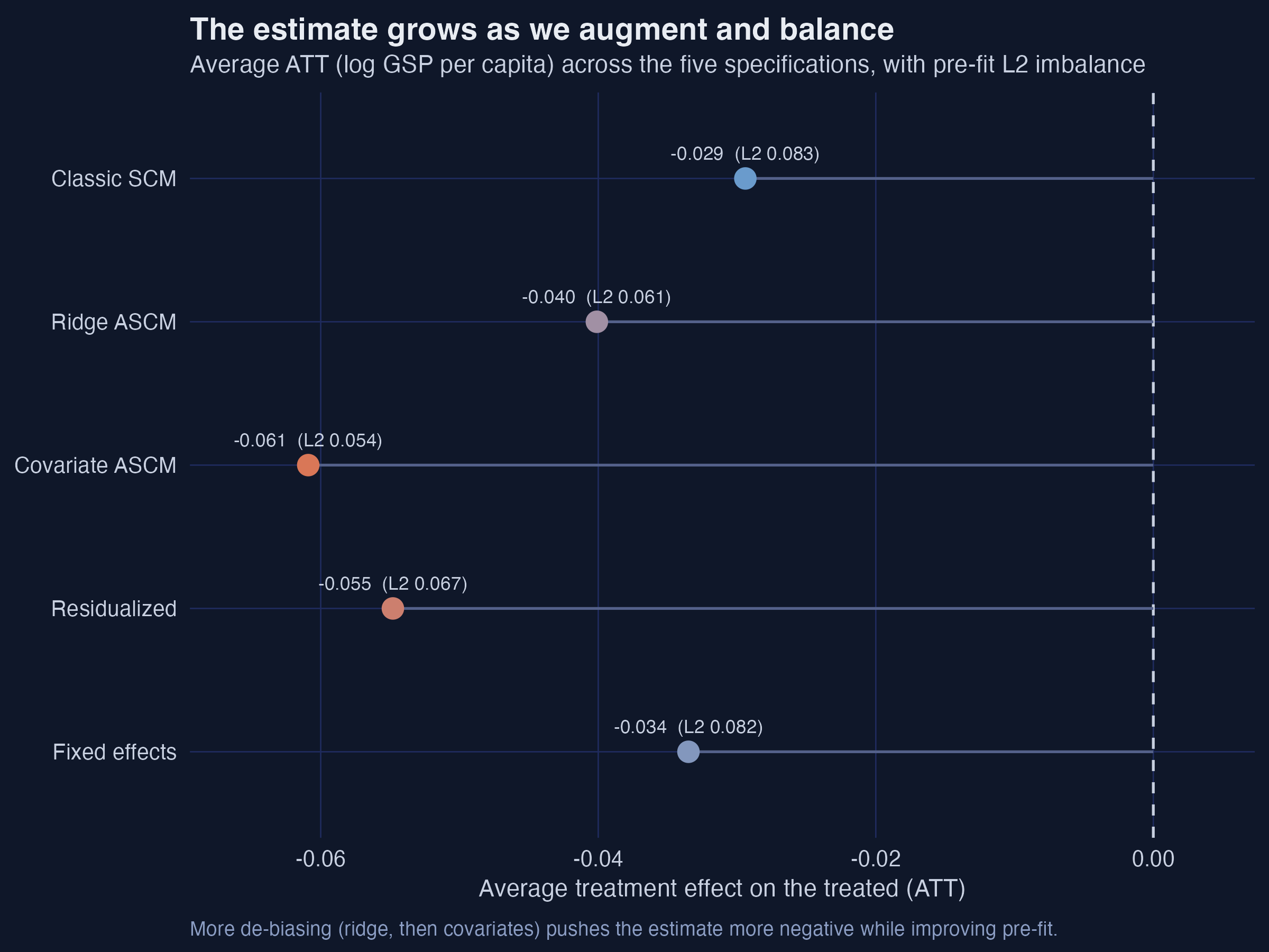
Interpretation. Read down the ladder of methods, a consistent pattern emerges: the more we de-bias and balance, the larger the measured damage. The ATT moves from −0.029 (classic SCM) to −0.040 (ridge) to −0.061 (covariate-augmented), while the pre-fit L2 imbalance falls from 0.083 to 0.062 to 0.054. The fixed-effect (−0.034) and residualized (−0.055) variants fall between these in magnitude. This monotonic pattern is reassuring rather than alarming: it tells us the un-augmented SCM estimate was the conservative one, understating the effect because of the very imbalance ASCM was designed to remove.
| Specification | ATT (log pts) | ≈ % effect | Pre-fit L2 | Est. bias |
|---|---|---|---|---|
| Classic SCM | −0.029 | −2.9% | 0.083 | — |
| Ridge ASCM | −0.040 | −3.9% | 0.062 | 0.011 |
| Covariate ASCM | −0.061 | −5.9% | 0.054 | 0.027 |
| Residualized | −0.055 | −5.3% | 0.067 | 0.006 |
| Fixed effects | −0.034 | −3.3% | 0.082 | — |
11. Discussion: what did the Kansas experiment do?
Putting the pieces together, the evidence points one direction: the 2012 Kansas tax cut is associated with a persistent shortfall in GDP per capita of roughly 3 to 6%, relative to a synthetic Kansas built from other states. The effect is strongest in 2013–2014, robust in sign across all five specifications, and — importantly — larger once we correct the bias that classic SCM leaves behind. The supply-side promise of accelerated growth does not appear in the data; if anything, Kansas underperformed its counterfactual.
Three caveats keep this honest. First, significance is genuinely borderline: depending on the inference method, the average effect either clears or just misses the 5% bar, even though individual 2013–2014 quarters are significant. We should describe this as suggestive-to-moderate evidence, not a knock-down result. Second, the estimate is the net gap, not a tax-only effect — Kansas also suffered a severe drought and aerospace-sector shocks over this window, which a synthetic control cannot separately strip out. Third, like all SCM analyses, the result rests on the assumption that a weighted blend of donors can stand in for Kansas’s untreated path, and that no other state was affected by Kansas’s policy.
For a policymaker, the practical takeaway is not a single number but a pattern: the better we make the comparison, the worse the tax cut looks, and at no point does it look good. That is a meaningfully different conclusion than “no detectable effect,” which is what a hasty reading of the classic-SCM p-value alone might have suggested.
12. Summary and next steps
What we did and found:
- Built a synthetic Kansas from a 7-state convex blend (classic SCM) and estimated a −2.9% post-2012 effect with a pre-fit imbalance of 0.083.
- Augmented with ridge regression to correct the imperfect pre-2012 fit, deepening the estimate to −3.9%, improving the fit to 0.062, and quantifying the SCM bias at 0.011 (≈ one-third of the effect) — all while moving the weights by a negligible RMS of 0.015.
- Added covariates to push the estimate to −5.9% with near-perfect covariate balance.
- Tested significance four ways and found a coherent but borderline picture: jackknife+ excludes zero, conformal and permutation hover around p = 0.07–0.10, and the leave-one-donor jackknife is the most cautious.
Limitations: a single treated unit and a modest donor pool limit statistical power; the estimate cannot separate the tax cut from contemporaneous shocks; and the conclusion depends on the credibility of the synthetic match.
Where to go next:
- Try other outcome models via
progfunc("gsyn","en", …) and compare. - Move to multiple treated units and staggered adoption with
multisynth, or multiple outcomes withaugsynth_multiout, in the companion post on Augmented Synthetic Control for Multiple Countries. - Run your own sensitivity checks: vary the donor pool, the pre-period length, and the test statistic in
summary(..., stat_func = ...).
12.1 Exercises
- In-time placebo. Re-fit Ridge ASCM pretending the tax cut happened in 2009 Q2 instead of 2012 Q2 (restrict the data to pre-2012 and set the fake treatment time). The estimated “effect” should be near zero. Why is this a useful check, and what would a large fake effect imply?
- The penalty dial. Re-fit with
min_1se = FALSEso cross-validation minimizes the error instead of applying the one-standard-error rule. How do λ, the pre-fit L2, and the estimate change? Explain the bias–variance trade-off you observe. - Inference under the microscope. For the classic-SCM fit, change the conformal test statistic with
summary(syn, stat_func = function(x) abs(sum(x))). How does the joint-null p-value change, and why might prioritizing the average post-treatment effect (rather than the sum of absolute effects) be more or less appropriate here?
13. References
- Ben-Michael, E., Feller, A., & Rothstein, J. (2021). The Augmented Synthetic Control Method. Journal of the American Statistical Association, 116(536), 1789–1803.
- Abadie, A., Diamond, A., & Hainmueller, J. (2010). Synthetic Control Methods for Comparative Case Studies. Journal of the American Statistical Association, 105(490), 493–505.
- Abadie, A., & Gardeazabal, J. (2003). The Economic Costs of Conflict: A Case Study of the Basque Country. American Economic Review, 93(1), 113–132.
- Chernozhukov, V., Wüthrich, K., & Zhu, Y. (2021). An Exact and Robust Conformal Inference Method for Counterfactual and Synthetic Controls. Journal of the American Statistical Association, 116(536), 1849–1864.
augsynthpackage and the Kansas vignette: github.com/ebenmichael/augsynth.- Companion tutorial: Augmented Synthetic Control for Multiple Countries.
Carlos Mendez
Associate Professor of Development Economics
My research interests focus on the integration of development economics, spatial data science, and econometrics to better understand and inform the process of sustainable development across regions.