Difference-in-Differences for Regional Data

Did Medicaid expansion cut mortality? It depends who you weight by

+0.122unweighted 2x2 ATT

−2.563population-weighted · sign flip

2,604counties × 11 years

Carlos Mendez

Nagoya University (GSID)

July 8, 2026

The Tension

Act I

Same data, opposite answers — only the weights changed

Twenty million people gained Medicaid under the ACA’s staggered roll-out. Did fewer of them die?

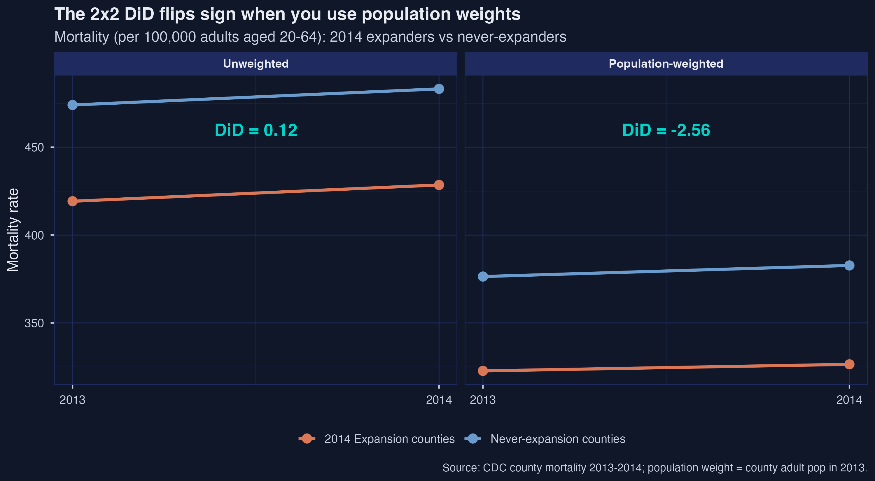
In the simplest four-cell DiD, unweighted says \(+0.12\) deaths per 100,000 (no help). Population-weighted says \(-2.56\) (lives saved). Which number is the answer?

This is the central tension of regional DiD. When units are counties that differ in size by three orders of magnitude — Los Angeles has more adults than Wyoming, Vermont and Alaska combined — weighting is not a precision knob, it changes the target parameter. The same arithmetic gives opposite signs.

The 2x2 DiD flips sign when you weight by population

Cell-means: 2014 expanders (orange) vs never-expanders (blue), unweighted (left) and population-weighted (right). Nearly parallel slopes on the left (DiD \(\approx 0\)), visibly divergent on the right (DiD \(\approx -2.6\)).

Spoiler figure — plant the reversal, don’t explain every panel yet. Treated trend +9.27 vs control +9.15 (unweighted, DiD +0.12); treated +3.74 vs control +6.30 (weighted, DiD −2.56). The pre-period gap is essentially identical across weightings (−54.77 vs −53.68), so the reversal is driven entirely by which counties dominate the averages, not by a level shift. We earn this picture across Act II.

Where we’re going

• The data: a 2,604-county, 11-year panel with staggered expansion timing
• The 2x2 — and why Levels = TWFE = Long-difference are one estimator
• Covariate adjustment: OR, IPW, doubly robust DRDID
• Modern staggered estimators: 2xT event study and Callaway–Sant’Anna
• HonestDiD: how fragile is the answer to pre-trend violations?

Teaching agenda built from the post’s learning objectives. The thread through all eight stages is the unweighted-vs-weighted contrast — we compute every estimate twice.

The Investigation

Act II

The estimand: an ATT whose weight is the question

\[\text{ATT}_\omega(2014) = \big(\mathbb{E}_\omega[Y_{2014}\mid D{=}1] - \mathbb{E}_\omega[Y_{2013}\mid D{=}1]\big) - \big(\mathbb{E}_\omega[Y_{2014}\mid D{=}0] - \mathbb{E}_\omega[Y_{2013}\mid D{=}0]\big)\]

The treated group’s change minus the control group’s change — both means taken under weighting scheme \(\omega\).

Equal weights \(\Rightarrow\) the typical treated county. Population weights \(\Rightarrow\) the typical treated adult. The subscript on \(\mathbb{E}_\omega\) carries the choice into the parameter itself.

Identification needs only one restriction: parallel trends — absent expansion, treated and control counties would have moved together. Everything in this deck is an ATT; the only quarrel is which weighted average of the unit-level effects we target.

Weighting shifts 11 points of mass between the two biggest cohorts

treat_year	counties	share counties	share adults (2013)
0 (never)	1,222	46.9%	38.2%
2014	978	37.6%	49.5%
2015 / 2016 / 2019	404	15.6%	12.4%

Population weighting rebalances toward large, urban 2014 expanders and small, rural never-expanders — a different comparison, not a tighter one.

This 11-point gap between county shares and population shares for the two largest cohorts is the proximate cause of the sign reversal. The three small cohorts shrink further under weighting. Switching the weight is switching the comparison.

On a balanced 2x2, Levels = TWFE = Long-difference — they are one estimator

# (a) levels: DiD is the interaction coefficient
feols(crude_rate_20_64 ~ D * Post, data = short_data, cluster = ~county_code)
# (b) two-way FE: same DiD, main effects absorbed
feols(crude_rate_20_64 ~ D:Post | county_code + year, cluster = ~county_code)
# (c) long difference: collapse to one row per county
feols(diff ~ D, data = short_long_diff, cluster = ~county_code)

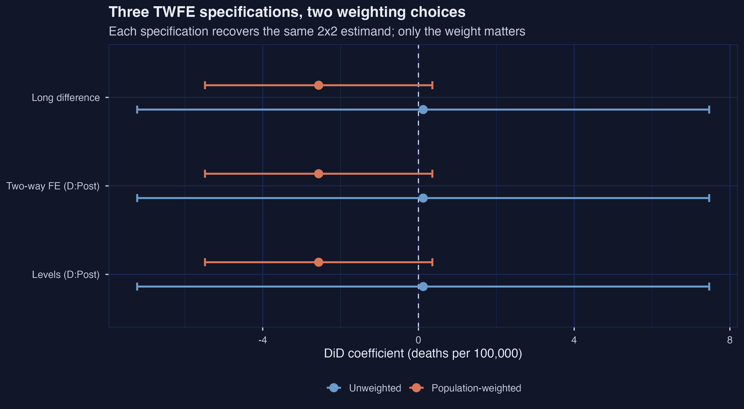
All three return \(+0.122\) unweighted and \(-2.563\) weighted — identical to three decimals.

This is the manuscript’s algebraic Result 1. For the 2x2 design there is no methodological choice between Levels, TWFE and Long-difference — they are the same estimator written three ways. The only substantive choice is whether to weight. Every later stage carries that lesson.

Three TWFE specs collapse onto two points — the form is interchangeable, the weight is not

Six DiD estimates (3 specs × 2 weights) with 95% CIs. The three rows within each weighting are superimposed; the weighting moves the point estimate by 2.7 deaths per 100,000.

Within a weighting the three specs are visually on top of one another. Across weightings the two colour groups separate cleanly. SEs differ across weights too: 3.75 unweighted vs 1.49 weighted (~2.5× tighter). The weighted CI [−5.48, +0.36] narrowly fails to exclude zero; the unweighted [−7.23, +7.47] is nowhere near.

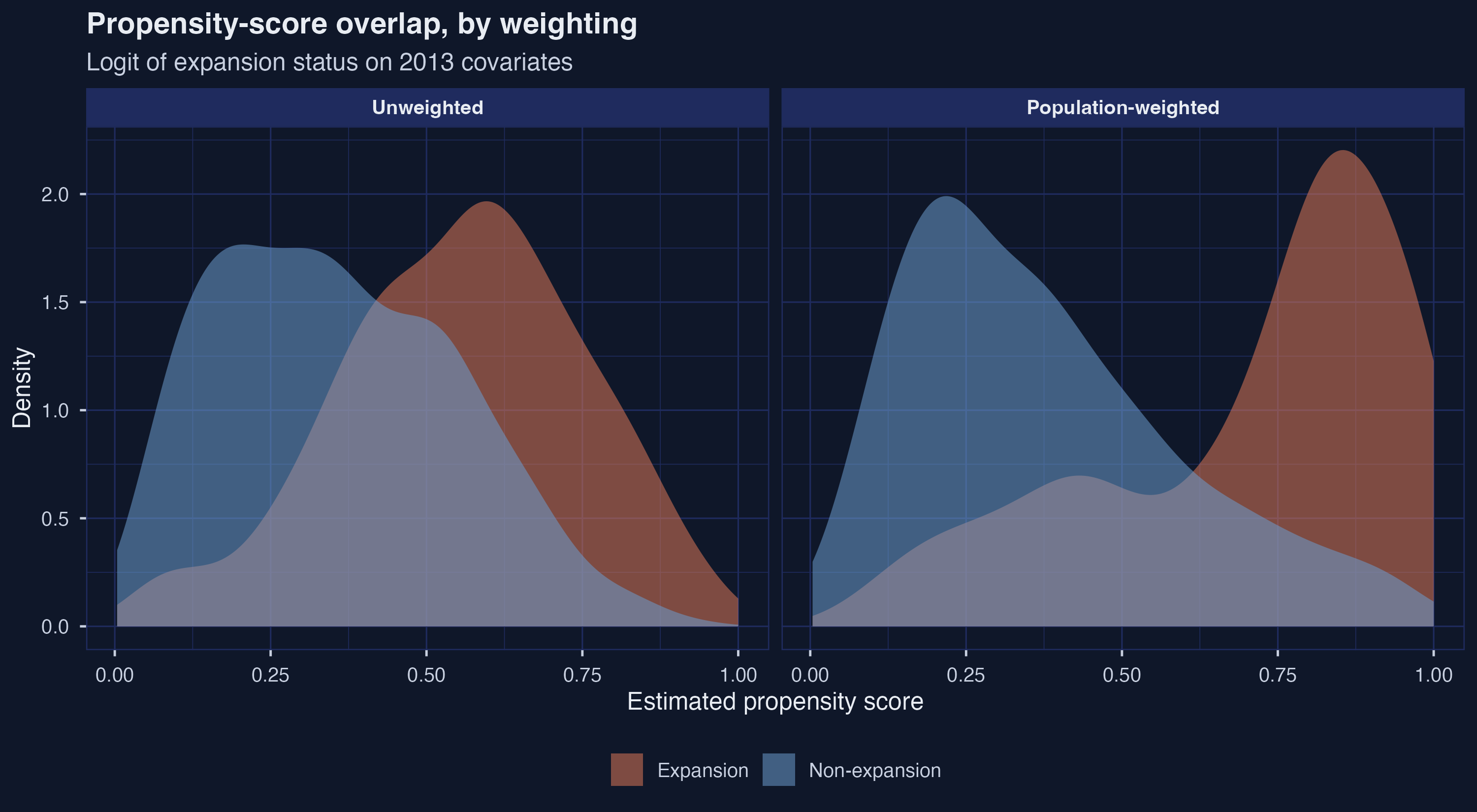
Expansion counties were whiter, richer, and worse-overlapping — so adjust

Propensity-score densities by expansion status, unweighted (left) and population-weighted (right). Weighting piles treated mass near \(0.85\) and spreads control mass bimodally — overlap gets worse, not better.

Six of twelve normalized-difference cells exceed the ±0.25 threshold. Unweighted: expansion counties whiter (+0.586), richer (+0.427), less poor (−0.423). Weighting shifts the imbalance toward unemployment (+0.503) and income (+0.685) because California and Texas pull the conditional means apart. Worse overlap is exactly why covariate adjustment matters more under weighting — and why we compute three adjusted estimators, not one.

Doubly robust DRDID is consistent if either model is right

\[\widehat{\text{ATT}}_{\text{DR}} = \frac{1}{n}\sum_{i=1}^{n}\big(\hat{w}_{D=1}(D_i) - \hat{w}_{D=0}(D_i, X_i)\big)\big(\Delta Y_i - \hat{\mu}_{\Delta, D=0}(X_i)\big)\]

Each county contributes a propensity-weighted residual: how far its 2013-to-2014 change strayed from the outcome model’s prediction for an untreated unit with the same covariates.

Belt-and-suspenders: the outcome model or the propensity model can be wrong — not both.

The “double” is that consistency survives misspecification of either the outcome regression or the propensity score, never requiring both. DRDID lands between OR and IPW because it is essentially a weighted combination of them.

Covariate adjustment nudges the point but the weighting gap survives intact

method	unweighted	population-weighted
Outcome regression (OR)	\(-1.615\)	\(-3.459\)
IPW	\(-0.859\)	\(-3.842\)
Doubly robust (DRDID)	\(-1.226\)	\(-3.756\)

Within-weighting spread \(\le 0.8\); across-weighting gap \(\approx 2.5\). None of the six 95% CIs excludes zero.

Adjustment moves the unweighted point from +0.12 (cell means) to −1.23 (DRDID) and the weighted from −2.56 to −3.76. Method and target parameter are orthogonal axes — and the second dominates. Note the causal framing: this is confounding control under observational identification, so covariates change the target parameter (unconditional ATT → ATT conditional on X), not just precision.

The 2x2 throws away nine years — the event study uses them all

The dynamic design estimates an \(\text{ATT}(e)\) for every year relative to expansion, with \(e = -1\) omitted as the baseline.

Leads (\(e \le -2\))

• Placebo for parallel trends
• Should hover near zero

Lags (\(e \ge 0\))

• Trace the effect over time
• Where the policy answer lives

We restrict to the 2014 cohort and never-treated counties — still no staggered cohorts yet — and aggregate the Callaway–Sant’Anna ATT(g,t) to event time. The leads double as a parallel-trends test; the lags are the dynamic treatment path.

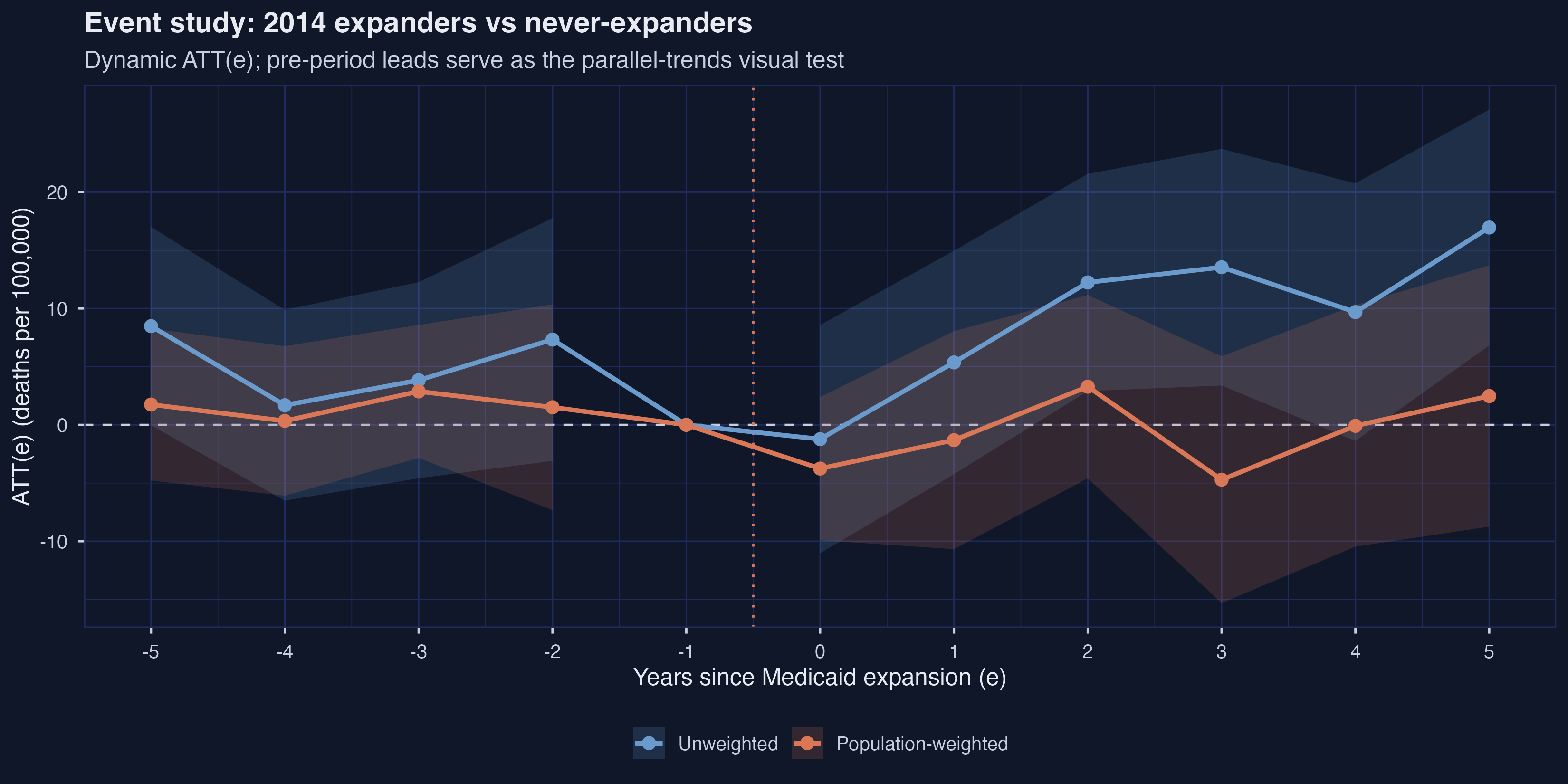
After expansion, the unweighted path climbs to +16.96 while the weighted stays flat

Dynamic \(\text{ATT}(e)\) for the 2014 cohort with shaded 95% CIs; dotted line at \(e=-0.5\) separates leads from lags. The two weightings track together pre-2014, then diverge sharply.

Unweighted ATT(e) climbs from −1.23 at e=0 to +16.96 at e=5, a CI of [+6.83, +27.09] that excludes zero — in the opposite-of-expected direction. Weighted ATT(e) wanders between −4.71 and +3.28 with every CI covering zero. The dynamic aggregate over e≥0 is +9.43 unweighted vs −0.68 weighted — a 10-death gap, far wider than the 2x2’s 2.7.

Callaway–Sant’Anna uses all the timing — one ATT(g,t) per cohort-year cell

\[\text{ATT}(g,t) = \mathbb{E}_\omega\big[Y_{i,t}(g) - Y_{i,t}(\infty)\mid G_i = g\big]\]

The effect of first expanding in year \(g\), relative to never expanding, evaluated at calendar time \(t\), restricted to units whose actual start year is \(g\).

Never make a mid-treatment unit serve as a “control” for an untreated one — the forbidden comparison that naive TWFE quietly makes.

\(G_i \in \{2014, 2015, 2016, 2019, \infty\}\). The design estimates a separate ATT(g,t) for each of 4×11 cohort-year cells, then aggregates — by cohort, or by event time. Identification is parallel trends with respect to the never-treated group, cohort by cohort.

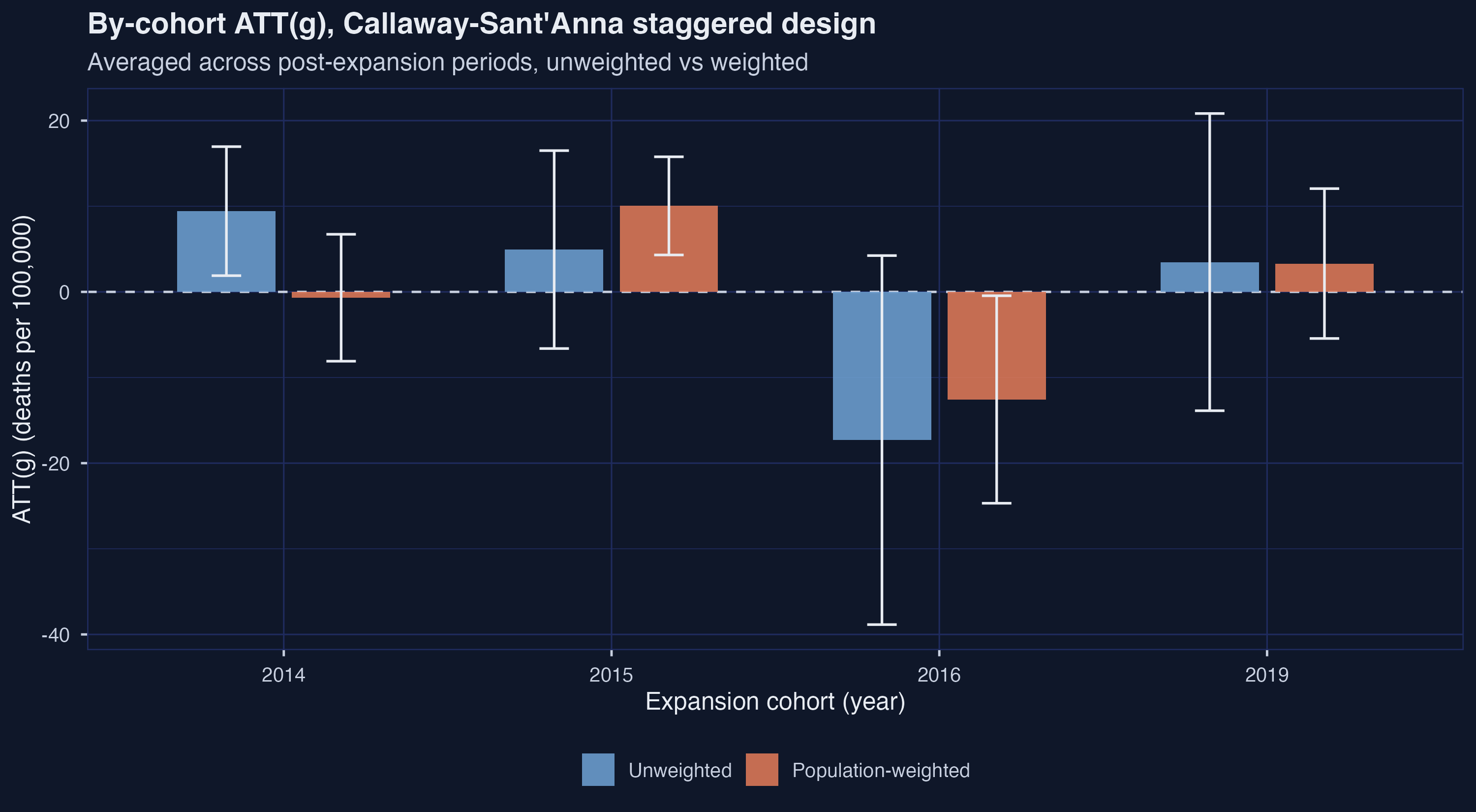
Four cohorts, four stories — the 2014 cohort flips sign with weighting

By-cohort \(\text{ATT}(g)\) bars with 95% CIs. The 2014 cohort flips (\(+9.43 \to -0.68\)); the 2016 cohort is the only weighted CI excluding zero (negative), on just 93 counties.

2014: +9.43 (significant) unweighted vs −0.68 (not) weighted — the manuscript’s verdict (“no significant change”) agrees with the weighted view. 2015: grows +4.94 → +10.04 (significant weighted). 2016: −12.57 weighted, CI excludes zero, but 93 counties carrying 2% of adults. 2019: one post-period, noisy. The manuscript warns these small cohorts may be “too noisy” — that caveat is doing real work.

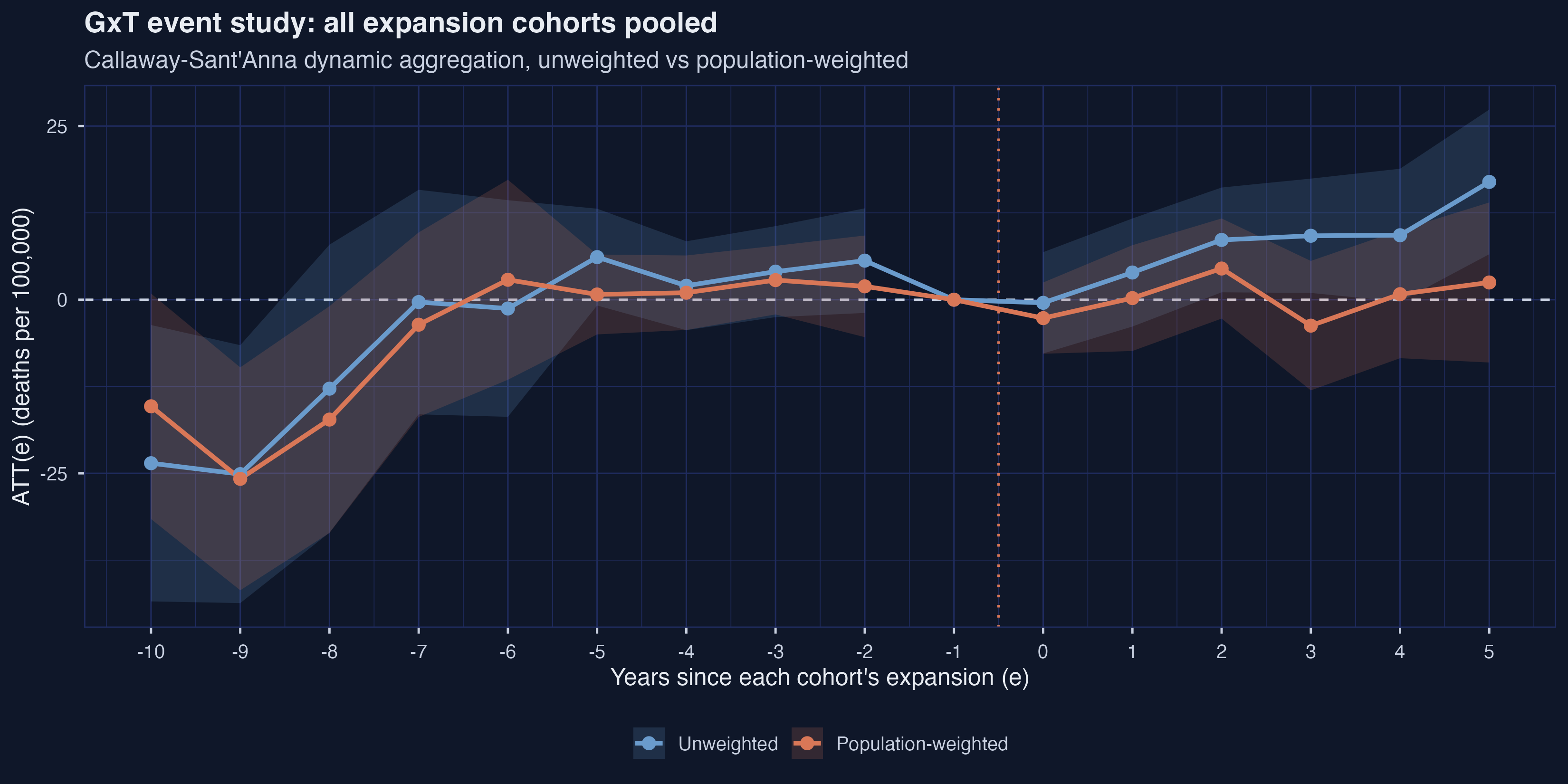
Pool the cohorts and the weighted dynamic path still hugs zero

GxT event study pooled across all four cohorts. Early leads (\(e=-10,-9\)) sharply negative (the lone 2019 cohort); from \(e=-7\) on, leads settle near zero; post-treatment the unweighted path reaches \(+16.96\) while the weighted stays within \(\pm 5\).

The dramatic e=−10/−9 leads (≈ −23 to −26, CIs excluding zero) are driven entirely by the small 2019 cohort — the only one with a pre-history that long. From e=−7 onward parallel trends are approximately restored. Pooling shrinks the weighting gap from 10.1 (2xT) to 7.7 (GxT) but does not flip the weighted sign: dynamic aggregate +7.92 unweighted vs +0.27 weighted.

The Resolution

Act III

The headline: weighting moves the answer by −2.56 deaths per 100,000

−2.56

the 2x2 ATT swings from \(+0.12\) (per county) to \(-2.56\) (per adult) — a sign flip with an identical pre-period gap

This is the single number to remember. The pre-period treated-minus-control gap is −54.77 unweighted, −53.68 weighted — essentially identical. So the reversal is not a level artifact; it is the weighted average targeting a different function of the same heterogeneous effects.

Across five stages, the weighting gap dwarfs the method gap

stage	unweighted	population-weighted	gap
2x2 cell-means / TWFE	\(+0.122\)	\(-2.563\)	\(2.69\)
2x2 DRDID	\(-1.226\)	\(-3.756\)	\(2.53\)
2xT dynamic (avg \(e\ge0\))	\(+9.428\)	\(-0.684\)	\(10.11\)
GxT dynamic (avg \(e\ge0\))	\(+7.917\)	\(+0.266\)	\(7.65\)

The gap is widest where staggered cohort heterogeneity is in play, narrowest where the 2x2 forces a single comparison.

The methodological choice between estimators within a row is always smaller than the choice between the two columns. That is the central pedagogical point of the whole pipeline, made quantitative.

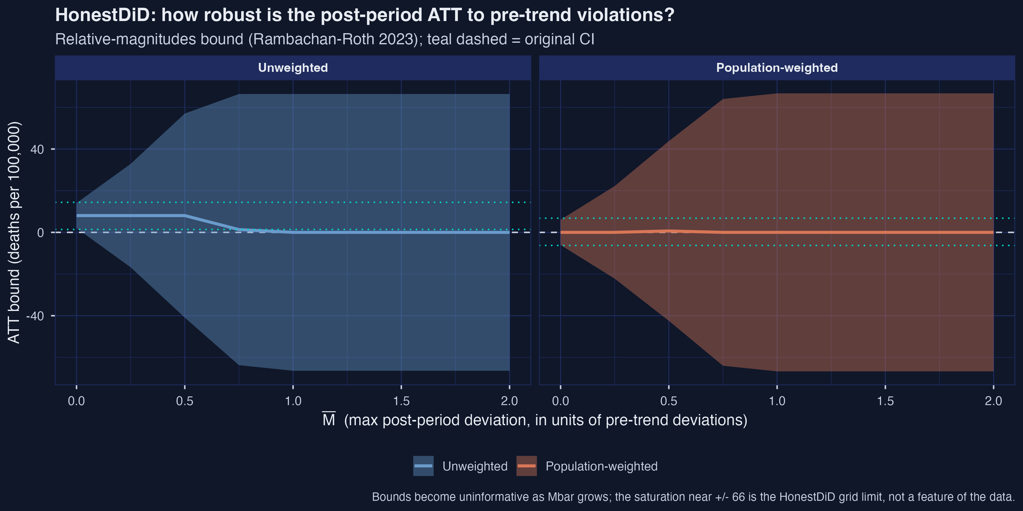
HonestDiD: every conclusion collapses by \(\bar{M} = 0.25\)

HonestDiD bounds across \(\bar{M}\), faceted by weighting. At \(\bar{M}=0\) the unweighted bound is all-positive \([+2.01, +14.09]\); the weighted straddles zero \([-6.07, +6.07]\). Both cross zero by \(\bar{M}=0.25\) and saturate at the grid limit (\(\pm 66\)) by \(\bar{M}=1\).

M-bar parameterizes the worst post-period parallel-trends violation as a multiple of the worst observed pre-period violation. The unweighted positive-sign conclusion breaks somewhere in the first quarter-multiple; the weighted result has no sign to break — its bound already covers zero at M-bar = 0. We learn very little from these pre-trends.

Does the staggered machinery make this causal? No — assumptions still carry the weight

Objection. Callaway–Sant’Anna and DRDID are modern, robust estimators — surely they pin down the effect.

Response. They fix the aggregation (no forbidden comparisons) and discipline selection on covariates — but identification still rests on parallel trends, and HonestDiD shows it is fragile here. The ATT is identified only under conditional parallel trends; the estimators cannot manufacture it.

Steelman, don’t strawman. Sun–Abraham / Callaway–Sant’Anna solve TWFE’s negative-weighting problem under staggered timing; DRDID solves covariate confounding under either model. Neither relaxes the identifying assumption. The manuscript explicitly flags this case as pedagogical, not a definitive Medicaid estimate.

Underpowered data, two estimands — not better and worse answers to one question

Per treated county

• unweighted GxT \(= +7.92\)
• 2xT reaches \(+16.96\) by \(e=5\)
• a heterogeneity object

Per treated adult

• weighted GxT \(= +0.27\)
• DRDID \(= -3.76 \pm 3.29\)
• the policy-relevant target

No CI excludes zero by a comfortable margin. When the policy is denominated in people, weight by people.

The cleanest answer the data support: not powerful enough to settle the question, and the unweighted and weighted estimands answer different questions. A federal cost-benefit assessment weights by adults; a study of which county types saw the largest local effects weights not at all. Both are legitimate — be explicit about which is on offer.

When units differ in size, choosing the weight is choosing the causal question.

The single takeaway. Weighting is not a precision detail in regional DiD — it selects the estimand. The unweighted answer is about counties; the weighted answer is about adults. Modern staggered estimators clean up the aggregation, but they cannot make the data more powerful or make one estimand the “right” one.