Spatial Inequality and the Kuznets Curve
Is there an inverted-U? A synthetic replication in R
Nagoya University (GSID)
June 15, 2026
Two pictures of the same question — and they disagree
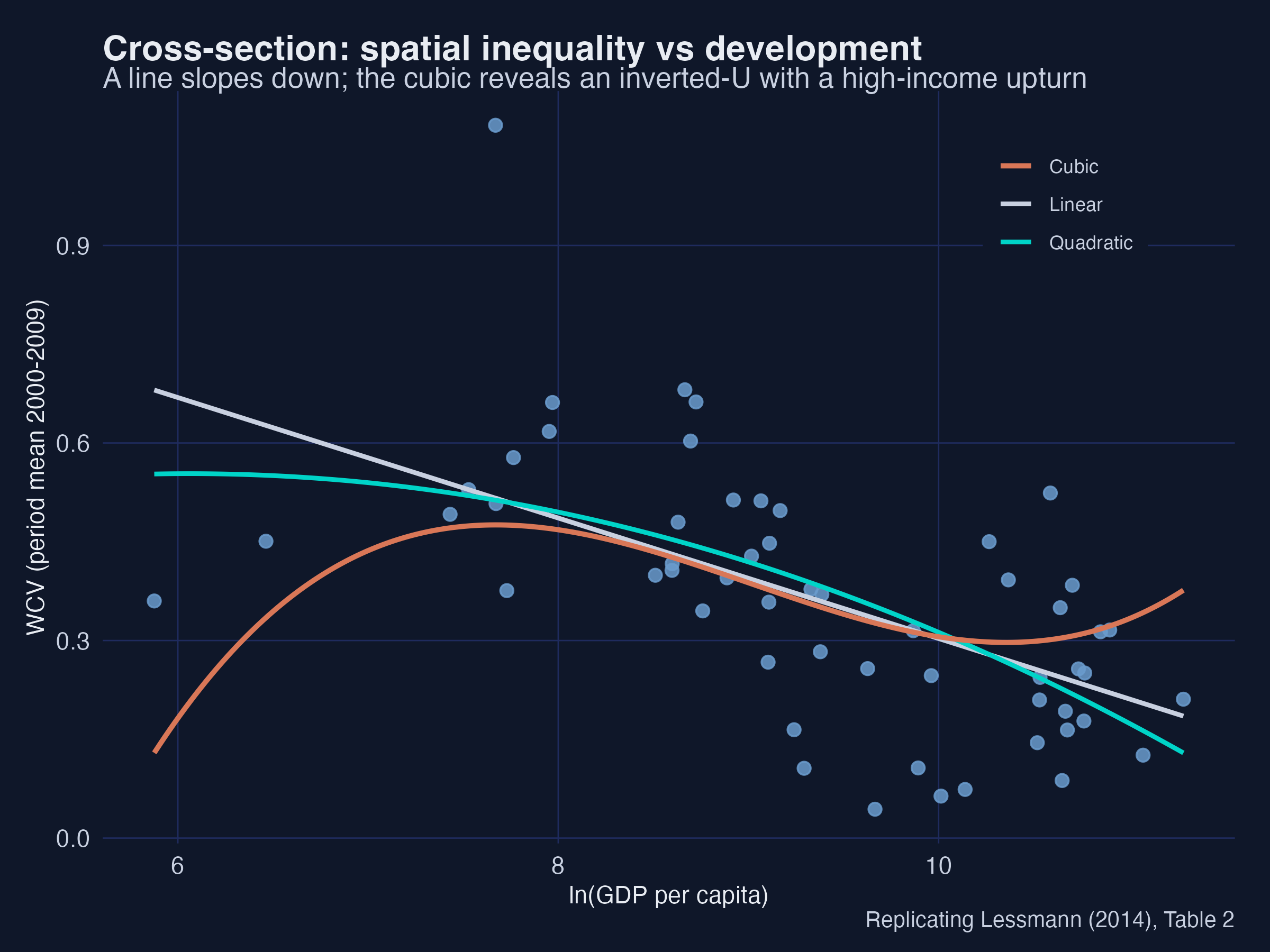
Cross-section: a line declines, a quadratic bends, a cubic adds a high-income upturn.
Spatial inequality is related to personal inequality — but not the same
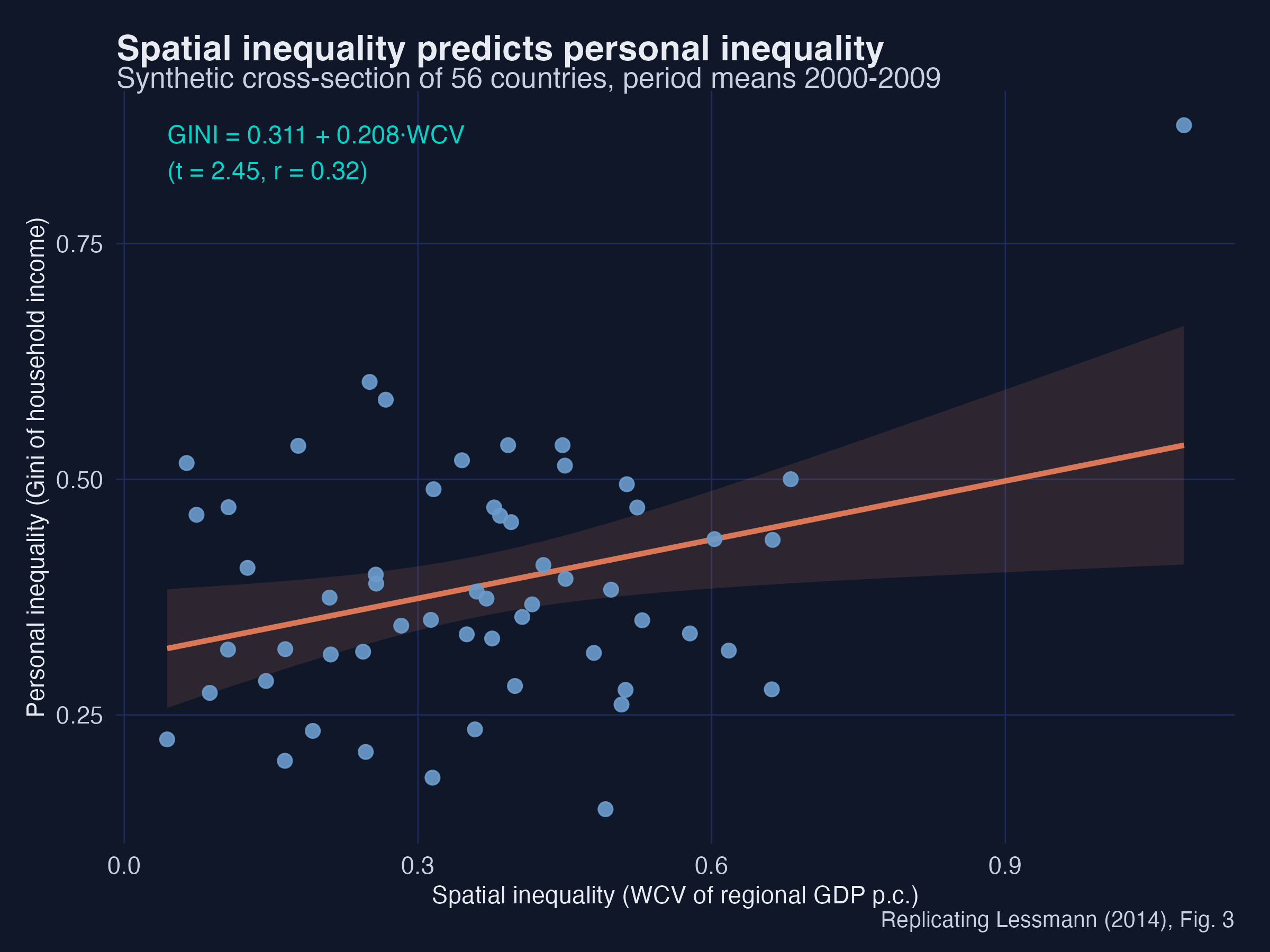
GINI = 0.31 + 0.21·WCV (t = 2.5, r = 0.32).
Cross-section: the inverted-U emerges with controls, and a cubic adds the upturn
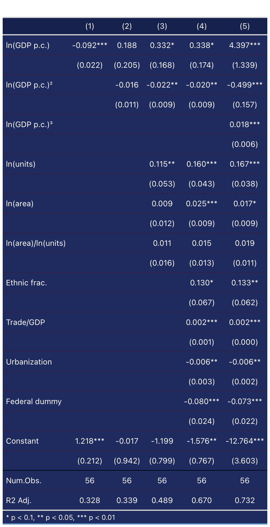
Five specifications: bivariate → quadratic → +controls (inverted-U) → +cubic (N-shape).
Where does the curve turn? Set the derivative to zero
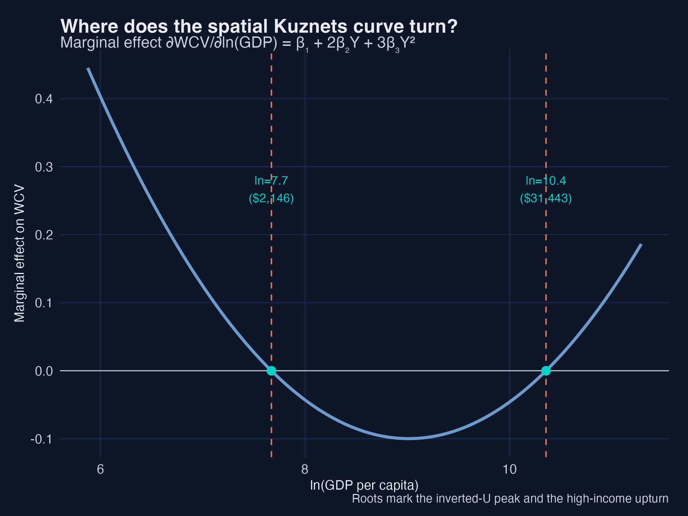
∂WCV/∂ln(GDP) = β₁ + 2β₂Y + 3β₃Y² = 0 → peak ≈ $2,100, trough ≈ $31,000.
The discriminant decides the shape
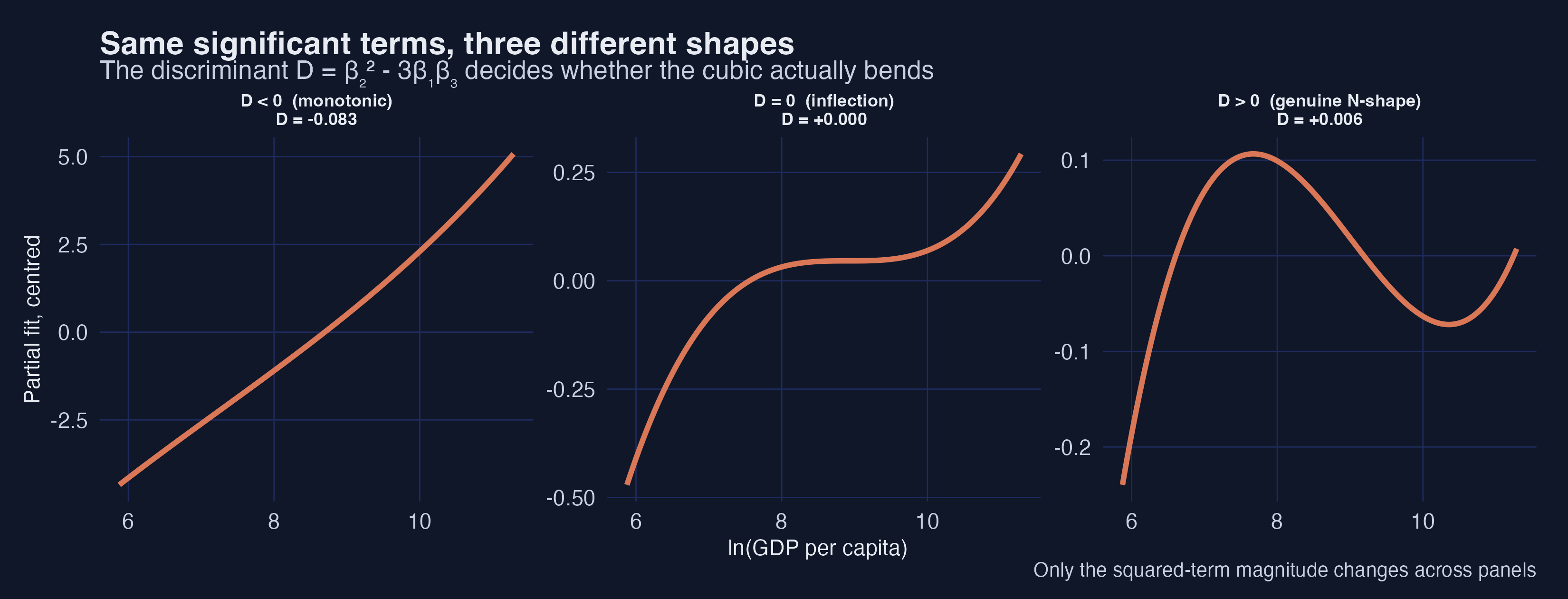
Same significant terms, three shapes — only the discriminant tells them apart.
The within-country inverted-U
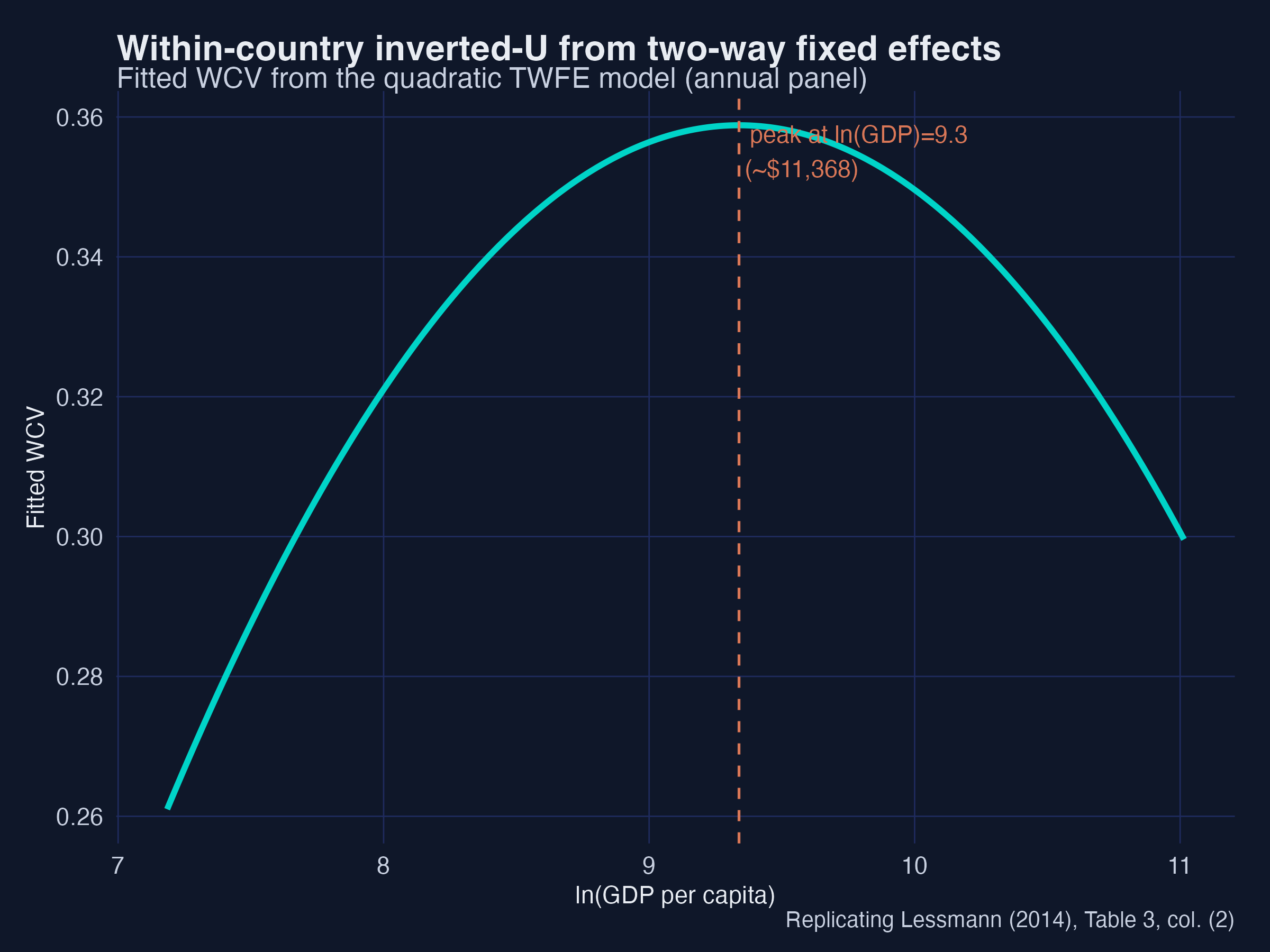
Fitted WCV from the two-way FE quadratic, peaking near $18,000.
Semiparametric, no polynomial assumed — same shape
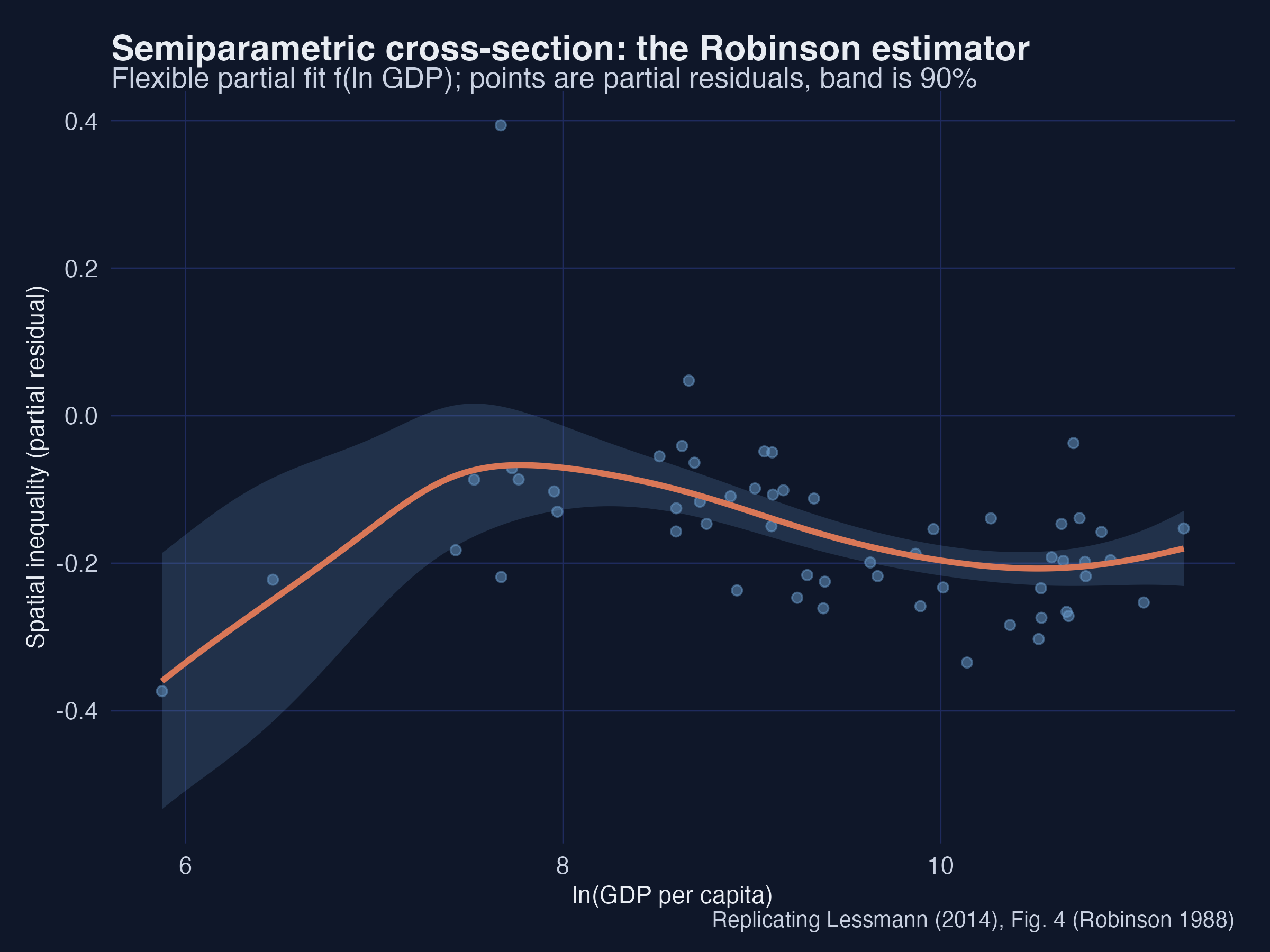
Robinson (1988) partial fit with a 90% band: inverted-U with a high-income upturn.
Structural change is the mechanism
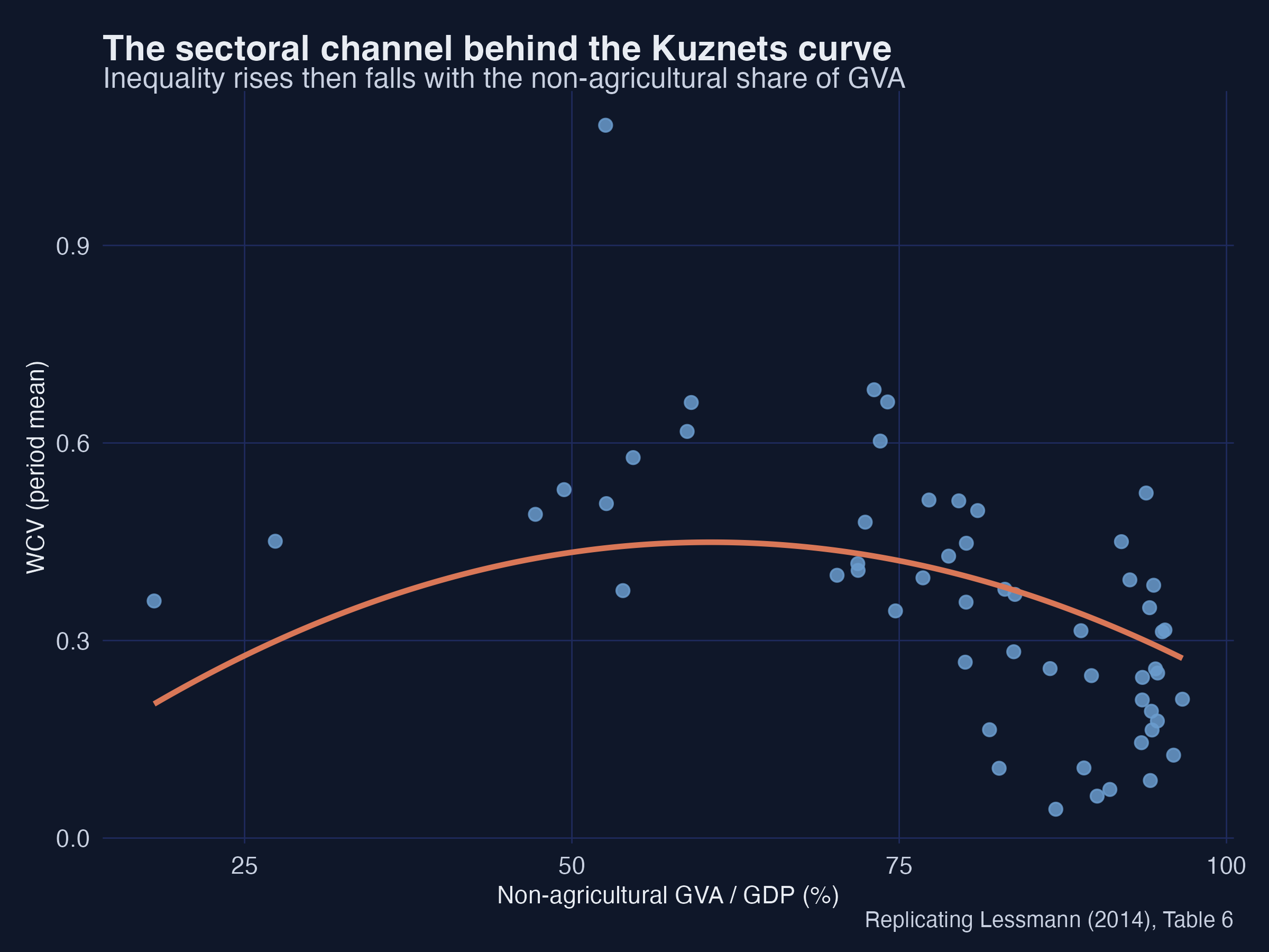
Replace income with the non-agricultural share of output — the inverted-U returns.
The high-income upturn is real but fragile
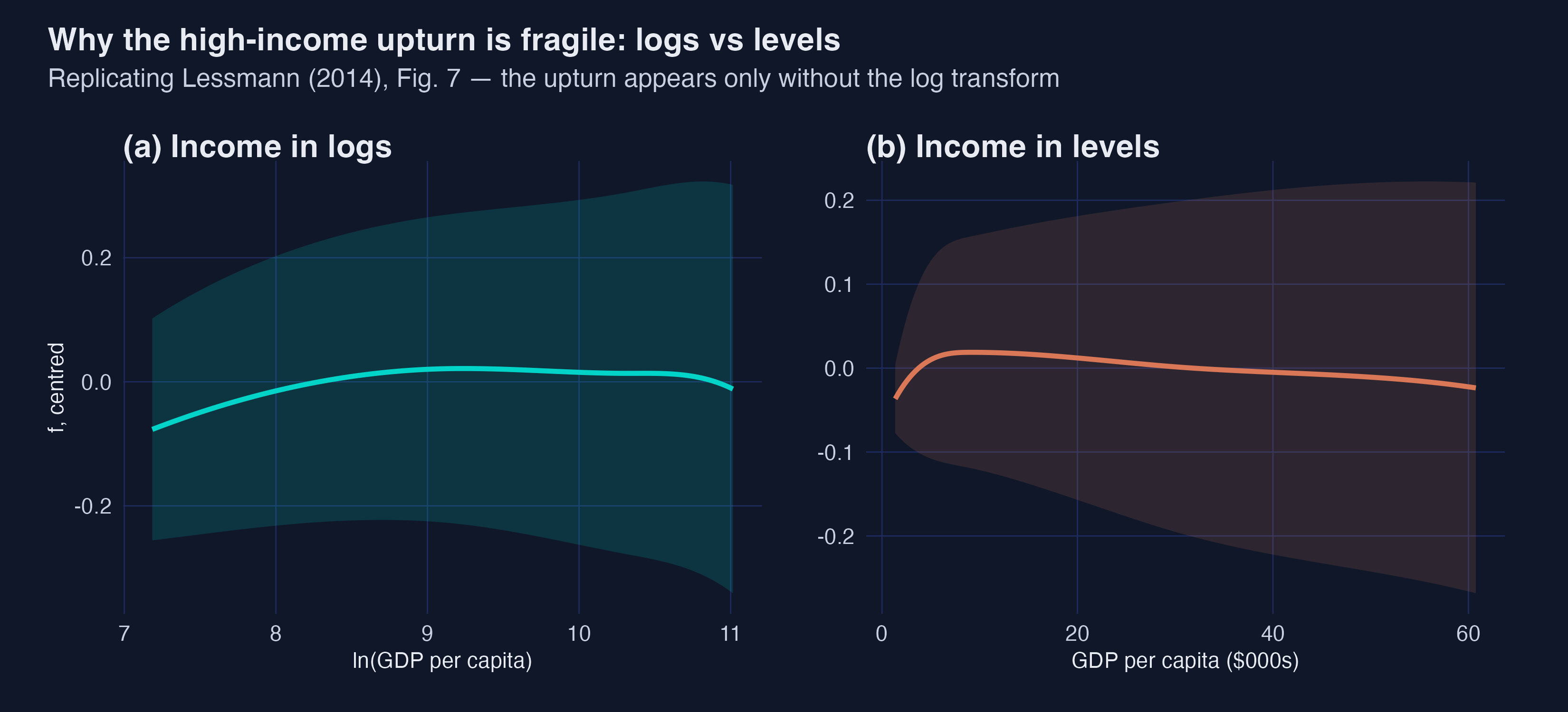
It appears in income levels, vanishes in logs (and within countries).