Augmented Synthetic Control for Multiple Countries: A Tutorial with augsynth

1. Overview

Did joining the euro make countries more productive? Did a national reform pay off, or would the country have done just as well without it? Questions like these share an awkward feature: we never observe the counterfactual — the path a country would have followed had it not adopted the policy. We see only the world that happened.

The synthetic control method (SCM) answers this by building the missing counterfactual from data. Among countries that did not adopt the policy, it finds the weighted recipe whose pre-treatment trajectory looks indistinguishable from the treated country’s, and uses that “synthetic” twin as the stand-in for the absent counterfactual. If the pre-treatment match is good, the post-treatment gap between the actual country and its synthetic version is the most credible estimate of the policy’s effect.

Classic SCM, however, has a well-known weak spot: it only works when the donor pool can reproduce the treated country’s pre-treatment path almost perfectly. In cross-country work the donor pool is small and countries are structurally different, so a good match is the exception, not the rule. The Augmented Synthetic Control Method (ASCM) of Ben-Michael, Feller, and Rothstein (2021) fixes this by adding an outcome model that estimates and removes the leftover bias when the pre-treatment fit is imperfect — the same doubly-robust idea behind augmented inverse-probability weighting. When the fit is already good, the augmentation does almost nothing; when it is poor, it rescues the estimate.

This tutorial is a hands-on tour of ASCM in a multi-country setting using the augsynth package. It has two parts. In Part 1 we work with simulated data where the true effect is known, so we can introduce the three augsynth entry points and verify that each one recovers the truth:

• single_augsynth — one treated unit (the building block),
• multisynth — many treated units with staggered adoption,
• augsynth_multiout — one treated unit with several outcomes.

We save the simulated panel to a CSV you can reuse, and we run a small suitability test that shows exactly where plain SCM fails and augmentation saves the day. In Part 2 we put the method to work on real data, qualitatively replicating Papaioannou (2021), “European monetary integration, TFP and productivity convergence,” which asks whether the 12 founding members of the euro area saw faster total factor productivity (TFP) growth than a synthetic counterfactual built from non-euro economies.

Learning objectives:

• Distinguish the three augsynth entry points and recognize which one a problem calls for
• Read the augsynth formula mini-language (outcome ~ treatment | covariates)
• Use simulated data with a known effect to validate a causal estimator before trusting it on real data
• Explain when augmentation (the Ridge outcome model) matters and when it does not
• Replicate the qualitative findings of a published synthetic-control paper and compare estimates honestly
• Use augsynth’s inference toolbox — jackknife+, conformal, jackknife, and the wild bootstrap — and explain what makes an estimated effect statistically significant

The diagram below maps the three functions onto one pipeline.

flowchart TD
    P["Panel of countries<br/>(unit, time, outcome, treatment)"] --> D{"How many treated units?<br/>How many outcomes?"}
    D -->|one unit, one outcome| S["single_augsynth"]
    D -->|many units, staggered| M["multisynth"]
    D -->|one unit, many outcomes| O["augsynth_multiout"]
    S --> W["SCM weights W<br/>(convex recipe of donors)"]
    M --> W
    O --> W
    W --> R["+ Ridge outcome model<br/>(bias correction)"]
    R --> A["ATT = actual − synthetic"]
    A --> I["Inference<br/>jackknife+ / conformal / bootstrap"]
    style P fill:#6a9bcc,stroke:#141413,color:#fff
    style D fill:#f5f5f5,stroke:#141413,color:#141413
    style S fill:#d97757,stroke:#141413,color:#fff
    style M fill:#d97757,stroke:#141413,color:#fff
    style O fill:#d97757,stroke:#141413,color:#fff
    style W fill:#6a9bcc,stroke:#141413,color:#fff
    style R fill:#00d4c8,stroke:#141413,color:#141413
    style A fill:#00d4c8,stroke:#141413,color:#fff
    style I fill:#6a9bcc,stroke:#141413,color:#fff

The routing is by shape, not difficulty: count the treated units and the outcomes, and the panel flows to one of the three functions. All three then converge on the same machinery — a synthetic counterfactual built from convex donor weights, optionally refined by the Ridge bias-correction step, with the ATT read off as actual minus synthetic.

Key concepts at a glance

This post leans on a small vocabulary repeatedly. Each concept below has three parts. The definition is always visible; the example and analogy sit behind clickable cards — open them when a term feels slippery, leave them collapsed for a quick scan.

1. Synthetic control method (SCM). A weighted average of donor (untreated) units, built so that its pre-treatment path matches the treated unit. The synthetic’s post-treatment trajectory is the estimated counterfactual; the gap to the actual unit is the treatment effect (ATT).

2. Augmented SCM (ASCM) and bias correction. Plain SCM is only unbiased when the pre-treatment fit is (near) perfect. ASCM fits an outcome model on the donors and subtracts the part of the gap that model predicts — a bias correction. If the fit is already perfect the correction is zero; if not, it removes leftover imbalance.

3. Donor pool and convex weights $W$. The donors are the untreated units the synthetic is built from. The weights are non-negative and sum to one (a convex combination), so the synthetic is an interpolation, never an extrapolation, of the donors.

4. Prognostic (outcome) model — progfunc. The model ASCM uses to predict each unit’s untreated outcome. progfunc = "None" gives plain SCM; progfunc = "ridge" fits a Ridge regression on lagged outcomes and is the default, because it also supports valid confidence intervals.

5. Staggered adoption and partial pooling — multisynth, nu. When many units adopt at different times, multisynth fits one synthetic control per treated unit and partially pools them. The pooling knob nu runs from 0 (each unit separate) to 1 (one shared control); augsynth picks it automatically.

6. Multiple outcomes — augsynth_multiout. One treated unit can be tracked on several outcomes at once. A single set of donor weights is chosen to balance all outcomes jointly, which borrows strength across correlated series.

7. Inference: an augsynth toolbox. A point estimate is only half the answer; we also need to know whether it is distinguishable from zero. augsynth offers several tools. For a single unit we report the robust jackknife+ confidence interval (inf_type = "jackknife+") and the conformal p-value (inf_type = "conformal"); for many units, multisynth offers a jackknife interval and the more conservative wild bootstrap (inf_type = "bootstrap"); for multiple outcomes, conformal returns a p-value per outcome. Section 9 makes this concrete.

2. Setup

augsynth is not on CRAN, so we install it from GitHub (pinned to a specific commit for reproducibility). We also load Synth (a dependency), haven (to read the Stata file in Part 2), and the usual tidyverse plotting tools. Everything below was executed with R 4.5.2, augsynth 0.2.0, and Synth 1.1.10.

# augsynth is installed from GitHub (run once):
# remotes::install_github("ebenmichael/augsynth@7a90ea4")

library(augsynth)
library(haven)     # read the Stata .dta in Part 2
library(dplyr)
library(tidyr)
library(ggplot2)

set.seed(20260605)

# Site colour palette
STEEL_BLUE  <- "#6a9bcc"   # synthetic control
WARM_ORANGE <- "#d97757"   # treated / actual
NEAR_BLACK  <- "#141413"   # truth / reference
TEAL        <- "#00d4c8"   # ridge-augmented / highlight

A note on the formula mini-language you will see throughout: augsynth takes outcome ~ treatment on the left, and optional matching covariates after a pipe, outcome ~ treatment | x1 + x2. The unit and time arguments name the panel’s identifier columns, and t_int is the intervention time (for the single-unit functions). The treatment column is a 0/1 indicator that turns on when treatment starts.

3. A two-country intuition example

Before any weighting machinery, here is the whole idea in two countries. We simulate a treated country, “Atlantia,” whose untreated path is a clean copy of a comparison country, “Borealis,” plus an injected effect that switches on in 2012 and grows by 1.5 units per year. Because Borealis is the counterfactual by construction, the gap after 2012 must equal the injected effect.

years   <- 2000:2023
t_int   <- 2012
trend   <- 40 + 1.2 * (years - 2000) + 3 * sin(2 * pi * (years - 2000) / 9)
control <- trend + rnorm(length(years), 0, 0.6)
true_effect <- ifelse(years >= t_int, 1.5 * (years - t_int + 1), 0)
treated <- trend + rnorm(length(years), 0, 0.6) + true_effect

mean(treated[years >= t_int] - control[years >= t_int])  # estimated gap
mean(true_effect[years >= t_int])                         # true effect

[1] 9.601    # estimated mean post-2012 gap
[1] 9.75     # true mean injected effect

The estimated post-2012 gap is 9.60 against a true mean effect of 9.75 — within 1.5%. This is synthetic control in its simplest possible form: a single, perfectly matched comparison. The figure makes the logic visible — the two lines are indistinguishable before 2012, then Atlantia pulls away by exactly the injected amount.

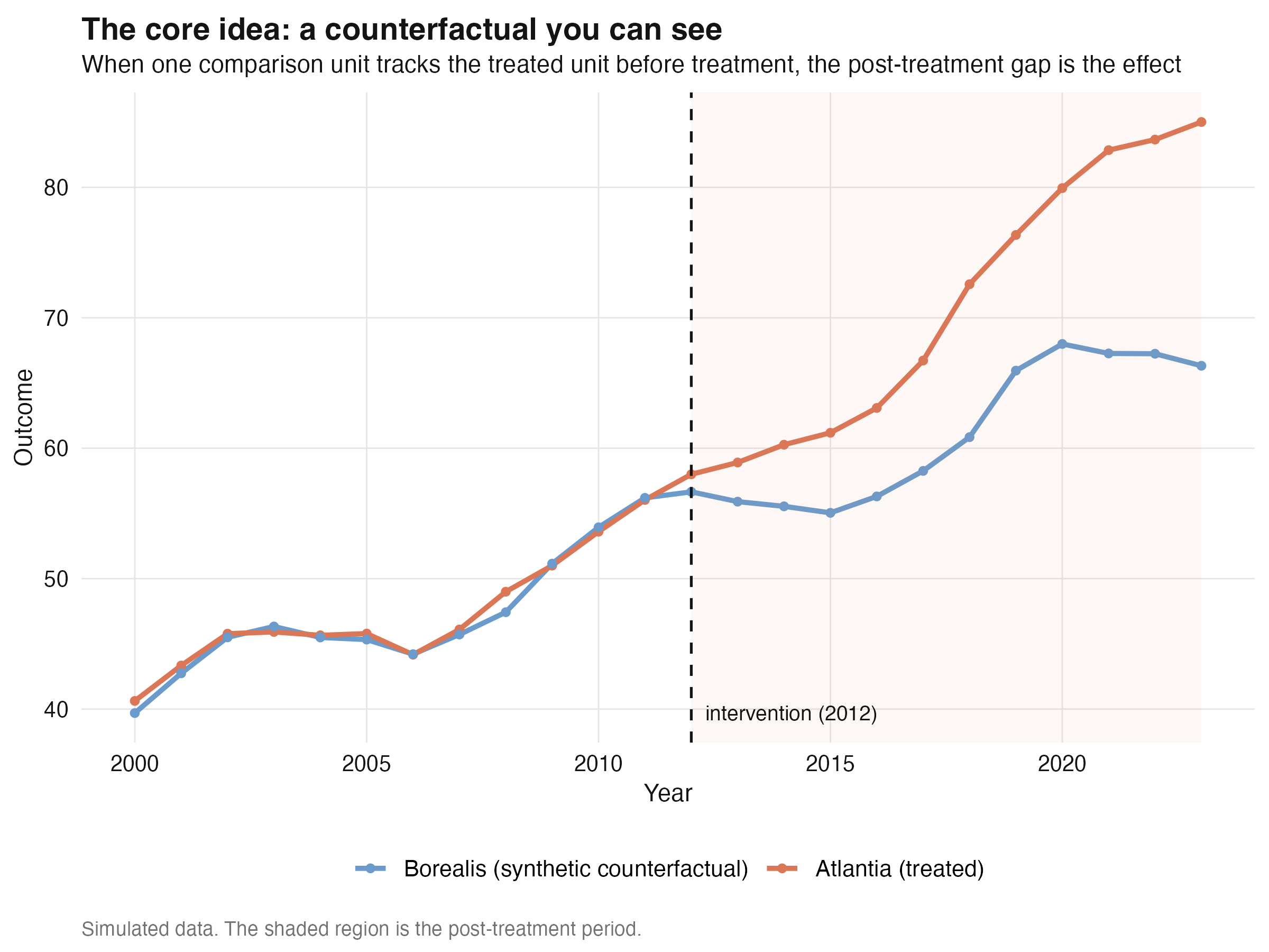
The catch, of course, is that real comparison countries are never perfect twins. That is why we need a weighted combination of many donors — and, when even that is not enough, the augmentation step. The rest of Part 1 builds up to both.

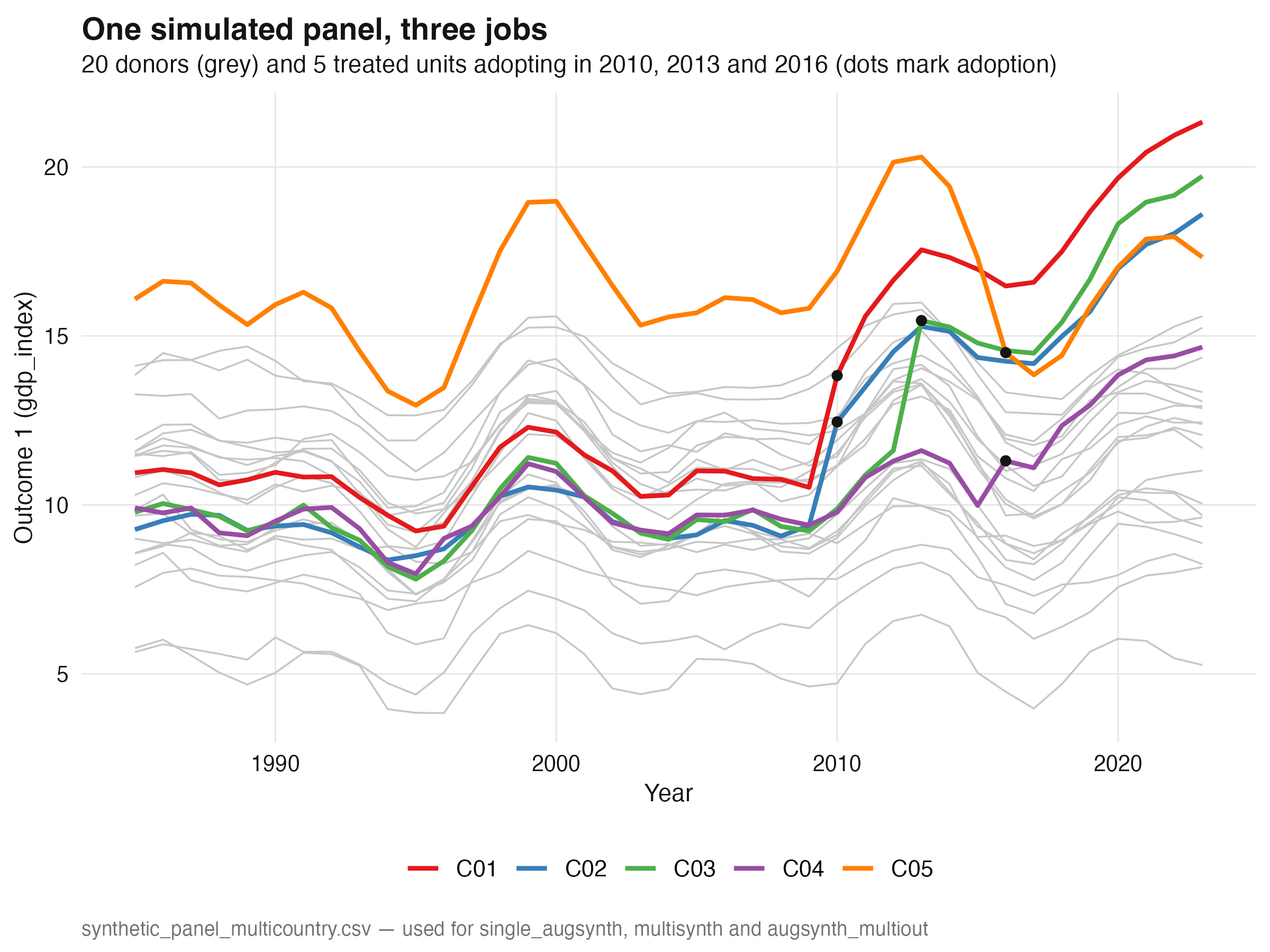
4. One reusable simulated panel

We now build a richer panel that all three functions will share. It has 25 countries over 39 years (1985–2023): five treated units (C01–C05) and twenty never-treated donors (C06–C25). The long pre-period is deliberate — it gives the inference procedures in Section 9 the statistical power they need. The data come from a three-factor model plus a unit fixed effect, so a good synthetic control genuinely exists. Treated units C01–C04 are each a sparse convex blend of three named donors (so a near-perfect synthetic control is guaranteed), while C05 is placed deliberately outside the donor hull to stress-test the methods later.

Treatment is staggered: C01 and C02 adopt in 2010, C03 in 2013, and C04 and C05 in 2016. The effect on the primary outcome gdp_index is a jump at adoption plus a gentle yearly ramp (with a correlated 0.6× effect on a second outcome trade_index). C01–C04 get large positive effects (a jump of +2.0 to +3.5 plus a +0.3 to +0.5 ramp); crucially, C05’s effect is small and negative (a −1.0 jump, −0.05 ramp), mimicking the real-world fact that a few euro members underperformed.

# ... factor-model construction (see analysis.R) ...
adopt <- c(C01 = 2010, C02 = 2010, C03 = 2013, C04 = 2016, C05 = 2016)
jump  <- c(C01 = 3.0, C02 = 2.5, C03 = 3.5, C04 = 2.0, C05 = -1.0)   # level shift
slope <- c(C01 = 0.5, C02 = 0.4, C03 = 0.5, C04 = 0.3, C05 = -0.05)  # yearly ramp

write.csv(panel, "synthetic_panel_multicountry.csv", row.names = FALSE)

Saved synthetic_panel_multicountry.csv: 25 units x 39 years = 975 rows
Adoption schedule: C01 2010  C02 2010  C03 2013  C04 2016  C05 2016
True outcome-1 jump at adoption: C01 3.0  C02 2.5  C03 3.5  C04 2.0  C05 -1.0
True outcome-1 yearly ramp:      C01 0.5  C02 0.4  C03 0.5  C04 0.3  C05 -0.05

The saved file ships with extra columns most real datasets never give you: the true counterfactual (gdp_index_cf, trade_index_cf) and the true injected effect (true_effect_gdp, true_effect_trade). Those let us grade every estimate against ground truth. Below, the twenty donor paths (grey) surround the five treated paths (colored), with dots marking each unit’s adoption year.

Two display equations capture what every augsynth call is doing under the hood. First, the SCM weight problem: find the convex donor weights $W$ that best match the treated unit’s pre-treatment vector.

$$W^{\star} = \arg\min_{W \in \Delta} \lVert X_1 - X_0 W \rVert_V \qquad \text{subject to} \qquad w_j \ge 0, \quad \sum_j w_j = 1$$

Here $X_1$ is the treated unit’s pre-treatment outcomes (and any covariates), $X_0$ is the matching donor matrix (one column per donor), $W$ is the vector of donor weights, $V$ weights the predictors, and $\Delta$ is the simplex (the constraint that weights are non-negative and sum to one). The solution $W^{\star}$ is the “recipe” for the synthetic control.

Second, the augmented, bias-corrected estimator. ASCM starts from the SCM gap and subtracts what an outcome model $\widehat{m}_t(\cdot)$ predicts the residual imbalance should be:

$$\widehat{\tau}_t^{\mathrm{aug}} = \Big(Y_{1t} - \sum_j w_j Y_{jt}\Big) - \Big(\widehat{m}_t(X_1) - \sum_j w_j \widehat{m}_t(X_j)\Big)$$

The first term is the ordinary SCM gap (actual treated minus weighted donors at time $t$). The second term is the correction: $\widehat{m}_t$ is the prognostic model (a Ridge regression when progfunc = "ridge"), evaluated at the treated unit’s covariates versus the donors’. When the pre-treatment fit is perfect the donors already reproduce $\widehat{m}_t(X_1)$, so the correction vanishes and ASCM equals SCM. When the fit is poor, the correction removes the leftover bias. This is the doubly-robust safety net.

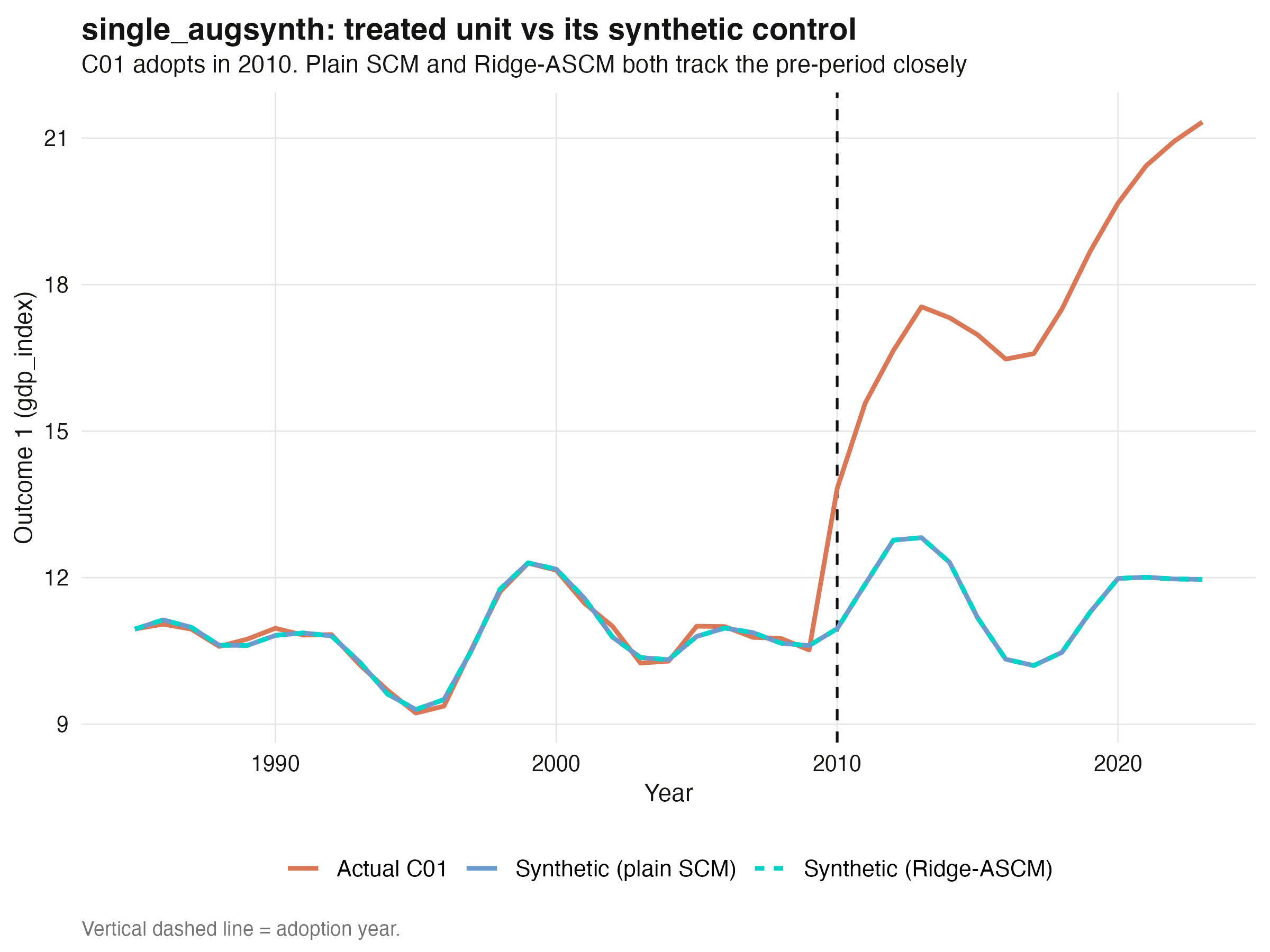
5. One treated unit: single_augsynth

The simplest case has one treated unit. We isolate C01 together with the twenty donors (never mixing in the other treated units — that would contaminate the donor pool), build the treatment indicator, and fit both plain SCM (progfunc = "None") and Ridge-ASCM (progfunc = "ridge"). The top-level augsynth() function dispatches to single_augsynth() automatically when it sees one treated unit and one intervention time.

sim_single <- panel |>
  filter(country %in% c("C01", donors)) |>
  mutate(trt = as.integer(country == "C01" & year >= 2010))

sc_plain <- augsynth(gdp_index ~ trt, country, year, sim_single,
                     t_int = 2010, progfunc = "None",  scm = TRUE)
sc_ridge <- augsynth(gdp_index ~ trt, country, year, sim_single,
                     t_int = 2010, progfunc = "ridge", scm = TRUE)

# jackknife+ confidence interval (robust) and conformal p-value
summary(sc_plain, inf_type = "jackknife+")$average_att
summary(sc_plain, inf_type = "conformal")$average_att

C01 true average post ATT : +6.250
Plain SCM  avg ATT : +6.241  jackknife+ [5.998, 6.506]  conformal p<0.001  L2=0.135
Ridge-ASCM avg ATT : +6.241  jackknife+ [5.998, 6.506]  conformal p<0.001  L2=0.135  lambda=2639

Both estimators nail the truth: the true average effect of C01 is +6.250 and each method returns +6.241, an error of 0.1%. And the effect is unambiguously real — the jackknife+ 95% confidence interval is [5.998, 6.506], comfortably excluding zero, and the conformal p-value is below 0.001. Notice that plain SCM and Ridge-ASCM give the same answer here. That is not a coincidence — C01 sits comfortably inside the donor hull, so the pre-treatment fit is already good (scaled L2 imbalance ≈ 0.14, well below the 1.0 you would get from naively averaging donors), and the Ridge penalty is driven to a large value (lambda ≈ 2639) that all but switches the augmentation off. This is the “when fit is good, ASCM ≈ SCM” principle in action.

The synthetic control reproduces C01’s pre-2010 path closely and then diverges, exactly as designed.

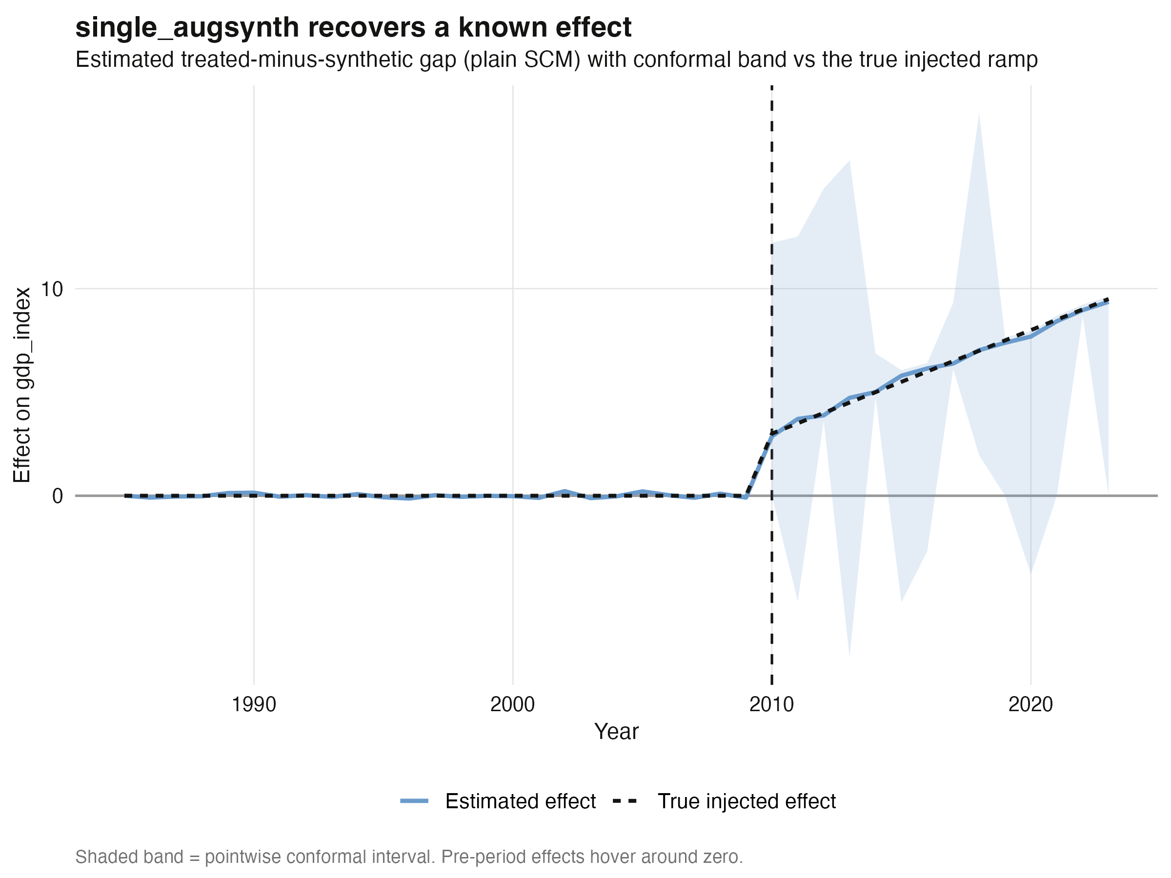
How well does the dynamic effect line up with the truth? The conformal gap plot overlays the estimated treated-minus-synthetic gap (with its pointwise band) against the true injected effect. The two are nearly on top of each other after 2010, while the pre-period gap hovers around zero — the visual signature of a trustworthy synthetic control.

The donor recipe is sparse and interpretable: synthetic C01 is built mostly from five donors (C19, C09, C13, C23, C08), with weights summing to one. This sparsity is a hallmark of SCM and makes the counterfactual auditable.

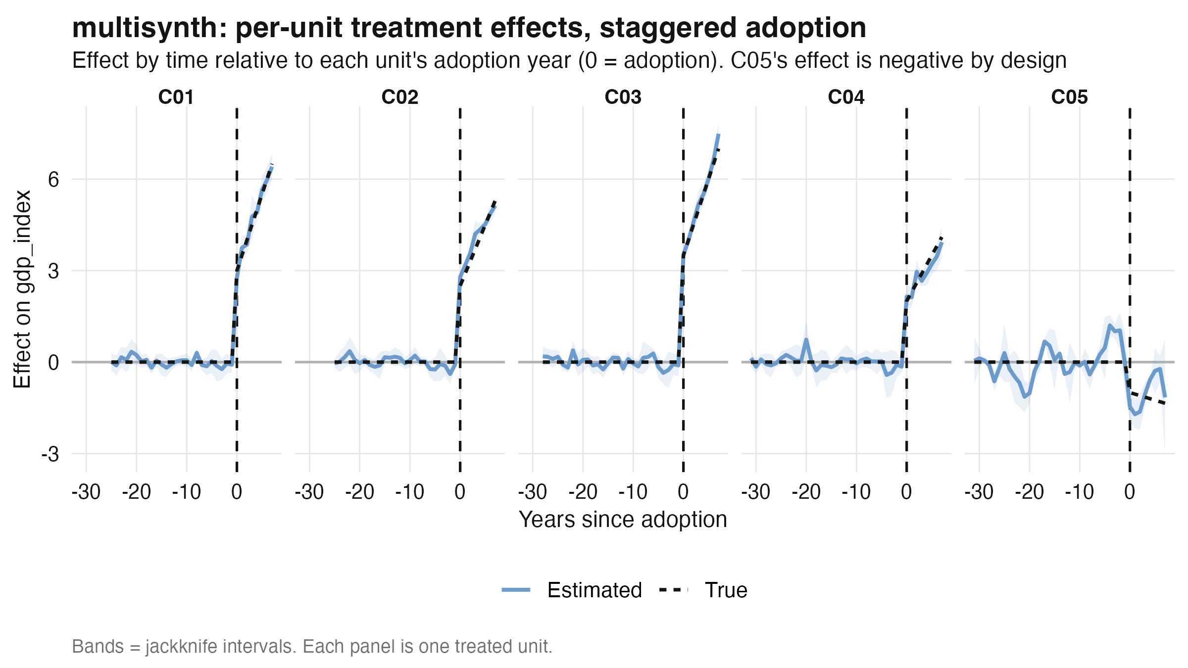
6. Many treated units, staggered adoption: multisynth

Real multi-country studies rarely have a single treated unit. multisynth handles many treated units that adopt at different times. It needs no t_int — it infers each unit’s adoption from when the treatment column switches from 0 to 1 — and it returns both a pooled average effect and per-unit effects, partially pooling them for stability.

sim_multi <- panel |>
  filter(country %in% c(treated, donors)) |>
  select(country, year, treat_ms, gdp_index)

ms_sim <- multisynth(gdp_index ~ treat_ms, country, year, sim_multi)
summary(ms_sim, inf_type = "jackknife")$att    # primary: tight interval
set.seed(20260605)
summary(ms_sim, inf_type = "bootstrap")$att     # conservative comparison

multisynth nu (auto) = 0.583 ; global scaled L2 = 0.052 ; n_leads = 8

Estimated vs TRUE average ATT (jackknife CI [ci_lo,ci_hi] + bootstrap CI [boot_lo,boot_hi]):
   level estimate  ci_lo ci_hi boot_lo boot_hi  truth
 Average    3.222  0.689 5.754  -2.468   9.779  3.155
     C01    4.756  4.461 5.050  -7.196  16.322  4.750
     C02    4.075  3.930 4.221  -6.000  13.800  3.900
     C03    5.362  5.154 5.570  -8.123  18.465  5.250
     C04    2.927  2.725 3.130  -4.499  10.072  3.050
     C05   -1.012 -1.639 -0.385 -3.039   1.195 -1.175

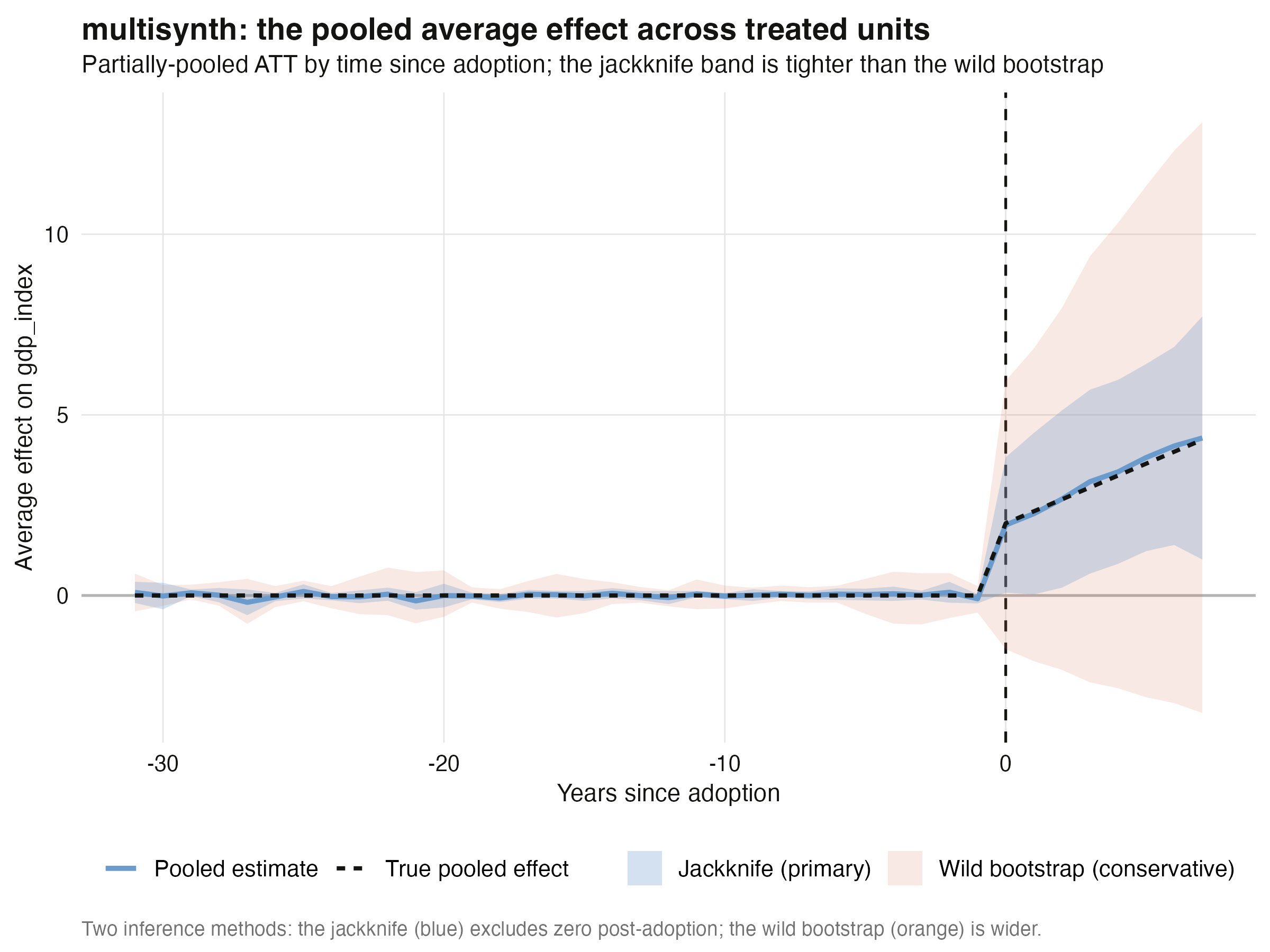
The pooled average effect is estimated at 3.222 against a true value of 3.155 — recovery to within 2%. Just as importantly, every per-unit estimate has the right sign and the right ballpark, including C05’s negative effect (−1.012 estimated vs −1.175 true). On the inference side, the jackknife confidence interval for the pooled effect is [0.689, 5.754], which excludes zero — the effect is significant. The more conservative wild bootstrap gives [-2.468, 9.779], which includes zero: same estimate, but it also propagates the counterfactual-estimation uncertainty, so it does not reach significance. This is our first concrete example of the inference method changing the verdict (Section 9 returns to it). The automatically chosen pooling parameter nu = 0.58 sits between “fully separate” and “fully pooled,” and the tiny global imbalance (scaled L2 = 0.05) tells us the joint synthetic controls fit the pre-period tightly. (One subtlety: multisynth averages effects over a common window of n_leads = 8 post-treatment periods so that all units contribute equally — which is why the per-unit estimates here, e.g. C01’s 4.756, are smaller than the full-period single_augsynth estimate of 6.241; we compute the truth over the same window to keep the comparison fair.)

The per-unit dynamics confirm the recovery. Each panel shows one treated unit’s estimated effect by time-since-adoption against its true effect; the pre-period sits at zero and the post-period jumps then climbs to meet the dashed truth line — with C05 dropping the opposite way.

Averaging across the five heterogeneous units gives the pooled effect path, the single most useful summary in a many-treated-unit study. The estimate tracks the true pooled effect closely, and the figure shows both inference bands — the tighter blue jackknife band (which excludes zero after adoption) and the wider orange wild-bootstrap band (which does not).

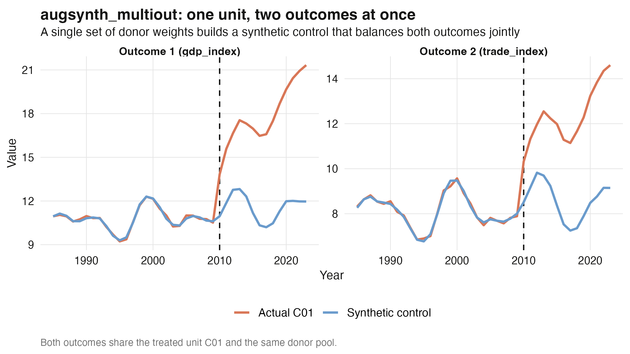
7. One unit, two outcomes: augsynth_multiout

Sometimes a policy plausibly moves several outcomes and we want one coherent counterfactual for all of them. augsynth_multiout puts multiple outcomes on the left of the formula, separated by +, and finds a single donor recipe that balances all of them before treatment.

mo <- augsynth_multiout(gdp_index + trade_index ~ trt, country, year,
                        t_int = 2010, sim_single,
                        progfunc = "None", scm = TRUE, combine_method = "avg")
summary(mo)$average_att   # conformal p-value per outcome

      Outcome  Estimate  p_val
1   gdp_index    6.538   <0.001     (true +6.250)
2 trade_index    3.531   <0.001     (true +3.750)

With a single set of weights, the joint fit recovers both effects: gdp_index at +6.538 (true +6.250) and the correlated trade_index at +3.531 (true +3.750), and both are significant (conformal p < 0.001 for each). The payoff of estimating them together — rather than running two separate single_augsynth fits — is that the donor weights must respect both series at once, which stabilizes the counterfactual when the outcomes are correlated. (A practical note on inference: augsynth_multiout’s summary() returns a conformal p-value per outcome but leaves the confidence-interval bounds as NA — a full CI needs grid_size > 1, which costs grid_size raised to the number-of-outcomes evaluations and, for effects this large, returns degenerate bounds. We therefore report the p-value.)

8. Testing suitability: where plain SCM fails and ASCM corrects

Now the payoff of building C05 outside the donor hull. No convex blend of the donors can reproduce its pre-treatment path, so plain SCM is in trouble. We fit both estimators for every treated unit and tabulate how far each lands from the known truth.

# fit plain and ridge for each treated unit; compare to known effects
recovery   # per unit: truth, plain, ridge, jackknife+ CI, conformal p, pre-fit L2, errors

 unit true_att att_plain att_ridge  ci_lo ci_hi p_plain sign_flip prefit_l2_plain err_plain err_ridge
  C01    6.250     6.241     6.241  5.998 6.506   0.000     FALSE           0.135     0.009     0.009
  C02    5.100     5.319     5.319  5.066 5.563   0.000     FALSE           0.150     0.219     0.219
  C03    6.000     6.282     6.282  5.958 6.624   0.000     FALSE           0.224     0.282     0.282
  C04    3.050     2.948     2.949  2.608 3.305   0.000     FALSE           0.258     0.102     0.101
  C05   -1.175     1.896    -1.145 -2.614 6.407   0.866      TRUE           0.414     3.071     0.030

Mean recovery error  — plain SCM: 0.737  | Ridge-ASCM: 0.128
C05 pre-fit scaled L2 — plain: 0.414  | ridge: 0.036 (lower = better fit)

This is the headline result of Part 1. For the four well-fit units (C01–C04), plain SCM lands within ~0.3 of the truth and its jackknife+ interval excludes zero (all significant; e.g. C01’s [5.998, 6.506]). For C05, plain SCM gets the sign wrong — it estimates +1.896 when the true effect is −1.175 — because it cannot match the pre-period and the unmatched bias swamps the signal. Its interval [-2.614, 6.407] includes zero (conformal p = 0.87): the estimate is both wrong and not significant, an honest double failure. Ridge-ASCM recovers −1.145, almost exactly right, by closing the pre-treatment gap (scaled L2 falls from 0.41 to 0.04). Across all five units, augmentation cuts the mean recovery error from 0.737 to 0.128. For the four well-fit units the two methods agree; augmentation earns its keep precisely on the hard case.

The picture says it all: under plain SCM the synthetic control (blue) drifts away from actual C05 (orange) before treatment — a fatal sign of poor fit — while Ridge-ASCM pins them together pre-2016, so the post-treatment gap can be trusted.

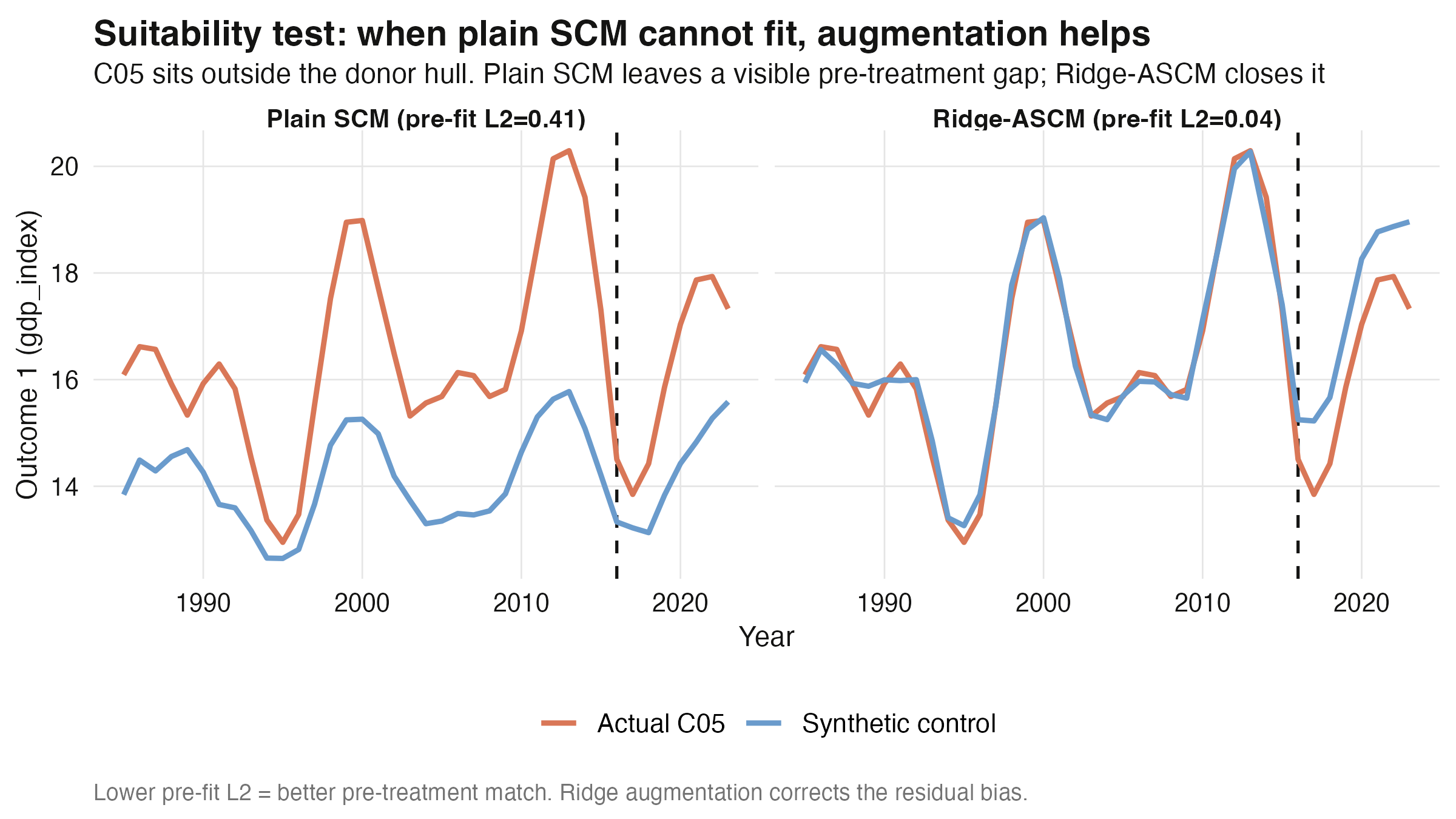
The practical rule: always read the pre-treatment fit. If the scaled L2 imbalance is small, plain SCM and ASCM will agree and either is fine. If it is large, trust the augmented estimate — and be suspicious of any synthetic control whose pre-period does not track.

9. Inference: is the effect real?

A point estimate answers “how big?”; inference answers “could this be noise?” A synthetic control gap is a difference between two estimated paths, so it carries uncertainty even when the point estimate is dead-on. augsynth ships several inference tools, and — this is the part most tutorials gloss over — they do not always agree. Choosing one and understanding what it measures is part of doing the method honestly.

The three tools, matched to the three estimators.

• single_augsynth → jackknife+ (primary) and conformal. The jackknife+ interval (summary(fit, inf_type = "jackknife+")) leaves out one donor at a time, refits, and builds a robust confidence interval for the average effect. We saw it call C01’s effect [5.998, 6.506] — comfortably away from zero. The conformal test (inf_type = "conformal") is a permutation procedure that returns a p-value and a pointwise band over time (the shaded band in the gap figures). It is powerful when the pre-period is long relative to the post-period — which is exactly why this panel starts in 1985, giving twenty-plus pre-treatment years — but its p-value is noisier and loses power when the post-window is long. With both tools agreeing here (jackknife+ CI excludes zero, conformal p < 0.001), we can trust the result.
• multisynth → jackknife (primary) and wild bootstrap. The jackknife is the natural interval for an average across treated units; on the simulated panel it put the pooled effect at [0.689, 5.754], significant. The wild bootstrap also propagates the counterfactual-estimation uncertainty, so it is wider — [-2.468, 9.779], not significant. The estimate is identical; the verdict is not. Neither method is “wrong”: the jackknife asks “is the average across these units different from zero?”, the bootstrap asks “accounting for how hard each counterfactual was to build, is it?” When they disagree, say so.
• augsynth_multiout → conformal. Returns a p-value per outcome (both < 0.001 for C01); a full confidence interval needs the slow grid_size > 1 path.

What drives significance. Three levers widen a confidence interval and can push a real effect below significance: more noise, fewer pre-treatment periods (a worse-pinned counterfactual), and a poorer pre-fit. This is the same lesson the suitability test taught from the other side — C05’s poor fit (scaled L2 = 0.41) gave it a wide interval that swallowed zero, while C01’s clean fit (L2 = 0.14) produced a tight, significant one. The interactive lab has a fifth tab, Inference, with a significance scoreboard and a slider-driven simulator: move effect size, noise, and the number of pre-periods and watch the interval widen or narrow and the verdict flip at the 5% line.

The honest-reporting rule. On simulated data, where we injected a real effect, every headline is significant. On the real euro-area data below, some results are and some are not — and we report them as they come, rather than dressing a near-zero effect up as a finding.

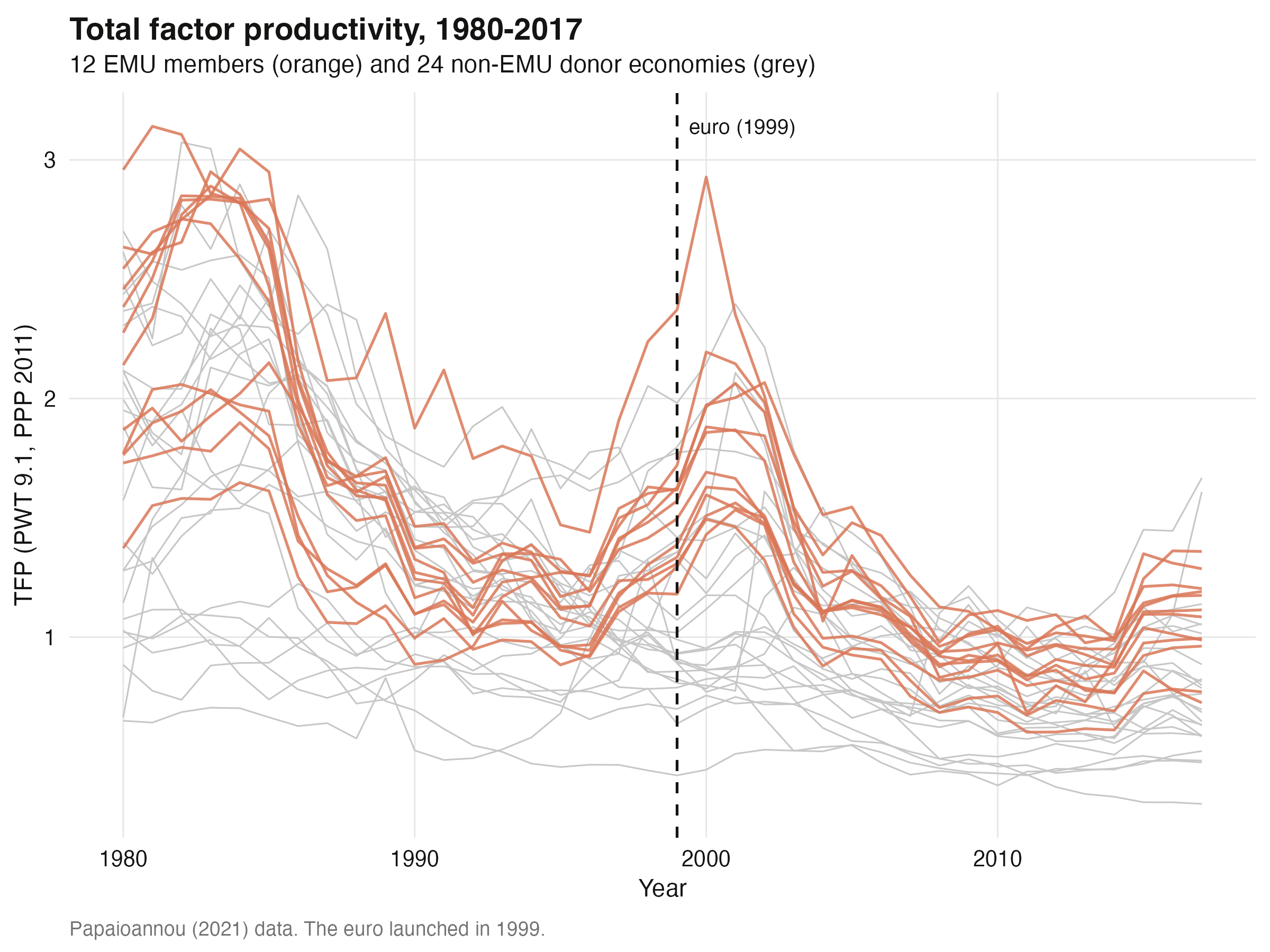
10. The EMU data: replicating Papaioannou (2021)

We now switch to real data. Papaioannou (2021) asks whether the euro raised the total factor productivity of its founding members. The dataset (shipped in this post’s reference/ folder as a Stata file) is a balanced panel of 36 countries from 1980 to 2017: the 12 founding euro members (Austria, Belgium, Finland, France, Germany, Greece, Ireland, Italy, Luxembourg, Netherlands, Portugal, Spain) and 24 non-euro donor economies (from Argentina to Uruguay). The primary outcome is tfp (total factor productivity from the Penn World Tables); a second outcome prod_gap is the log productivity gap versus the USA, where lower means closer to the frontier.

A subtlety worth pausing on: the file stores treat as a time-invariant group flag (1 for euro members in every year) and time1/time2 as period flags (post-1999, post-1992). The actual time-varying treatment is their product.

emu <- read_dta("reference/dataset_revision_1.dta") |>
  mutate(country = as.character(country)) |> zap_labels() |> as.data.frame()

emu$trt99 <- as.integer(emu$treat == 1 & emu$time1 == 1)  # euro members x post-1999
emu$trt92 <- as.integer(emu$treat == 1 & emu$time2 == 1)  # euro members x post-1992

EMU countries (12): Austria, Belgium, Finland, France, Germany, Greece, Ireland,
                    Italy, Luxembourg, Netherlands, Portugal, Spain
Donor countries (24): Argentina, Australia, Brazil, Canada, ... , Turkey, Uruguay

The raw TFP paths show the setup: twelve euro members (orange) embedded in a cloud of donors (grey), with the 1999 euro launch marked.

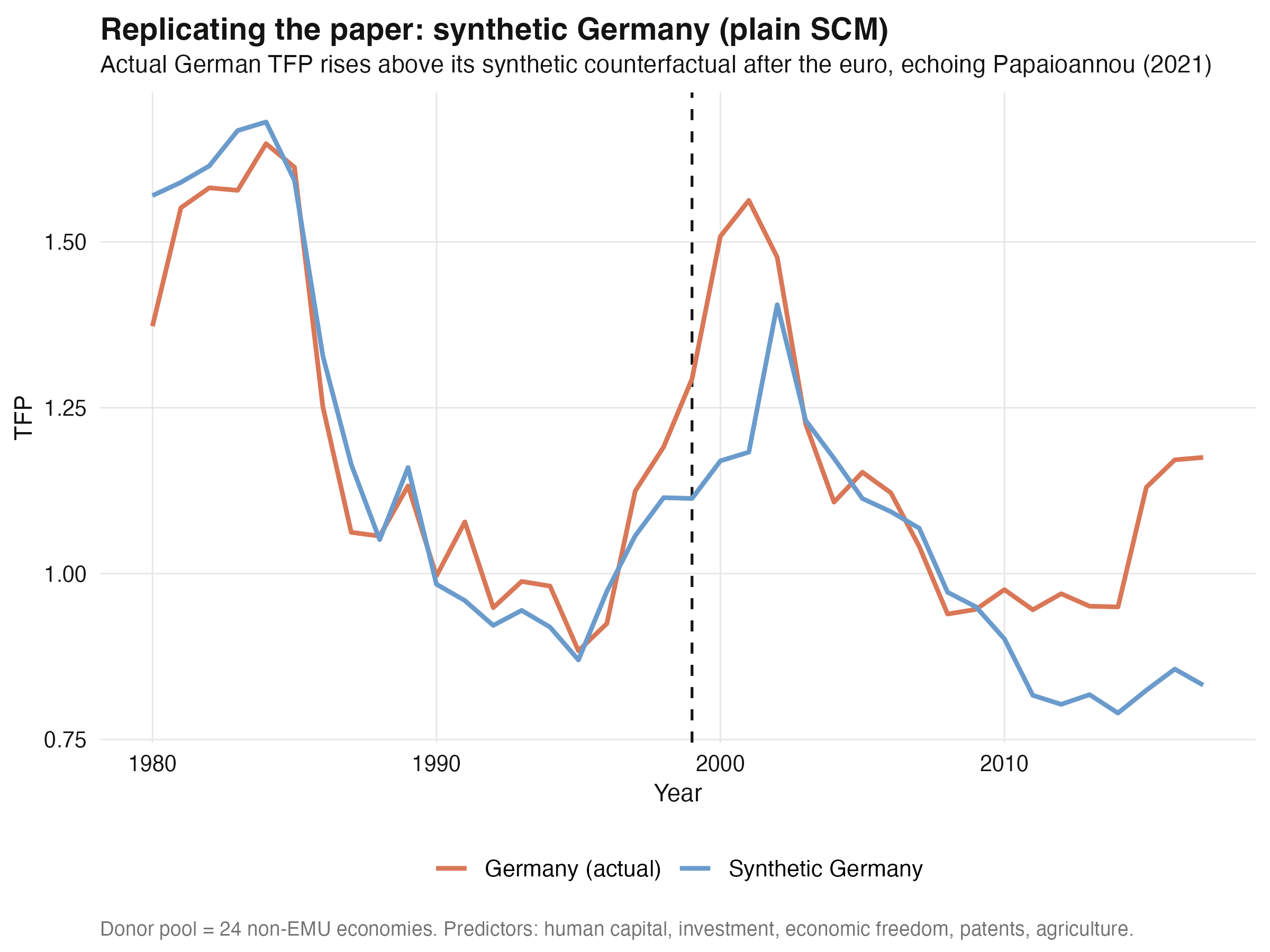
11. One country, the paper’s way: synthetic Germany (plain SCM)

We start with a single country to mirror the paper’s per-country synthetic controls. Germany is fit against the 24 donors, matching on pre-treatment TFP and the paper’s predictors (human capital, investment share, economic freedom, patents, agriculture share). This is plain SCM — the closest augsynth analogue to Abadie’s classic method.

fit <- augsynth(tfp ~ trt99 | hum_cap + inv_share + ec_freed + patents + agricult,
                country, year, germany_plus_donors, t_int = 1999,
                progfunc = "None", scm = TRUE)
summary(fit)$average_att

Germany plain SCM avg ATT (TFP): +0.133 | jackknife+ [-0.082, 0.336] | conformal p=0.027 | L2 0.301
Germany % effect — 2000-07: +8.0%   2008-17: +19.3%  (plain SCM)

Actual German TFP runs above its synthetic counterfactual after 1999, with an average effect of +0.133 TFP units — about +8.0% over 2000–2007 and +19.3% over 2008–2017. The pre-treatment fit is good (scaled L2 = 0.30). Here the two inference tools disagree at the margin, which is itself instructive: the conformal p-value is 0.027 (significant at 5%), but the jackknife+ interval [-0.082, 0.336] just barely includes zero. On real data with a modest effect, “significant” is genuinely borderline — we flag it rather than pick the answer we like. Qualitatively this still matches Papaioannou’s finding that Germany was among the clearer winners from monetary integration.

12. Ridge-ASCM as the modern extension

Does augmentation change the German verdict? We refit with progfunc = "ridge" and overlay the two counterfactuals.

fit_ridge <- augsynth(tfp ~ trt99 | hum_cap + inv_share + ec_freed + patents + agricult,
                      country, year, germany_plus_donors, t_int = 1999,
                      progfunc = "ridge", scm = TRUE)

Germany Ridge-ASCM avg ATT (TFP): +0.127 | conformal p=0.015 | scaled L2 pre-fit 0.292

The Ridge-augmented estimate (+0.127, conformal p = 0.015) is essentially the plain-SCM estimate (+0.133) — again, because the pre-treatment fit was already good (scaled L2 barely moves, 0.301 → 0.292). The two synthetic counterfactuals are nearly indistinguishable. This is reassuring rather than disappointing: augmentation is an insurance policy, and a quiet premium here means the classic estimate was already trustworthy for Germany.

13. All twelve members at once: multisynth

The multi-country headline uses multisynth to estimate the euro’s effect across all twelve members in one model. Because every member adopts in 1999, this is a simultaneous (block) design rather than a staggered one — multisynth handles it, it just does not exercise the staggered machinery we saw in Part 1.

ms_emu <- multisynth(tfp ~ trt99, country, year, emu_multi)
summary(ms_emu, inf_type = "jackknife")$att    # primary
set.seed(20260605)
summary(ms_emu, inf_type = "bootstrap")$att     # conservative comparison

Pooled EMU avg ATT (TFP): -0.016 | jackknife [-0.282, 0.250] | bootstrap [-0.259, 0.231] | global L2 = 0.100

Taken at face value, the pooled average effect is a near-zero −0.016, and it is not statistically significant — both the jackknife [-0.282, 0.250] and the wild bootstrap [-0.259, 0.231] comfortably include zero. (Unlike the simulated panel, where the two methods disagreed, here they agree: there is simply no pooled signal to detect.) But the single number is also misleading, and reading only the average would be a mistake: the dynamics are the real story. The pooled effect path is flat through the entire pre-period (no pre-trend — a good sign), rises to about +0.39 in the first euro years, then slides into negative territory during the 2008–2014 crisis before recovering toward zero by 2017. The early gains and the crisis losses cancel out in the long-run average. This dynamic — strong early, eroded by the crisis — is exactly the arc Papaioannou describes.

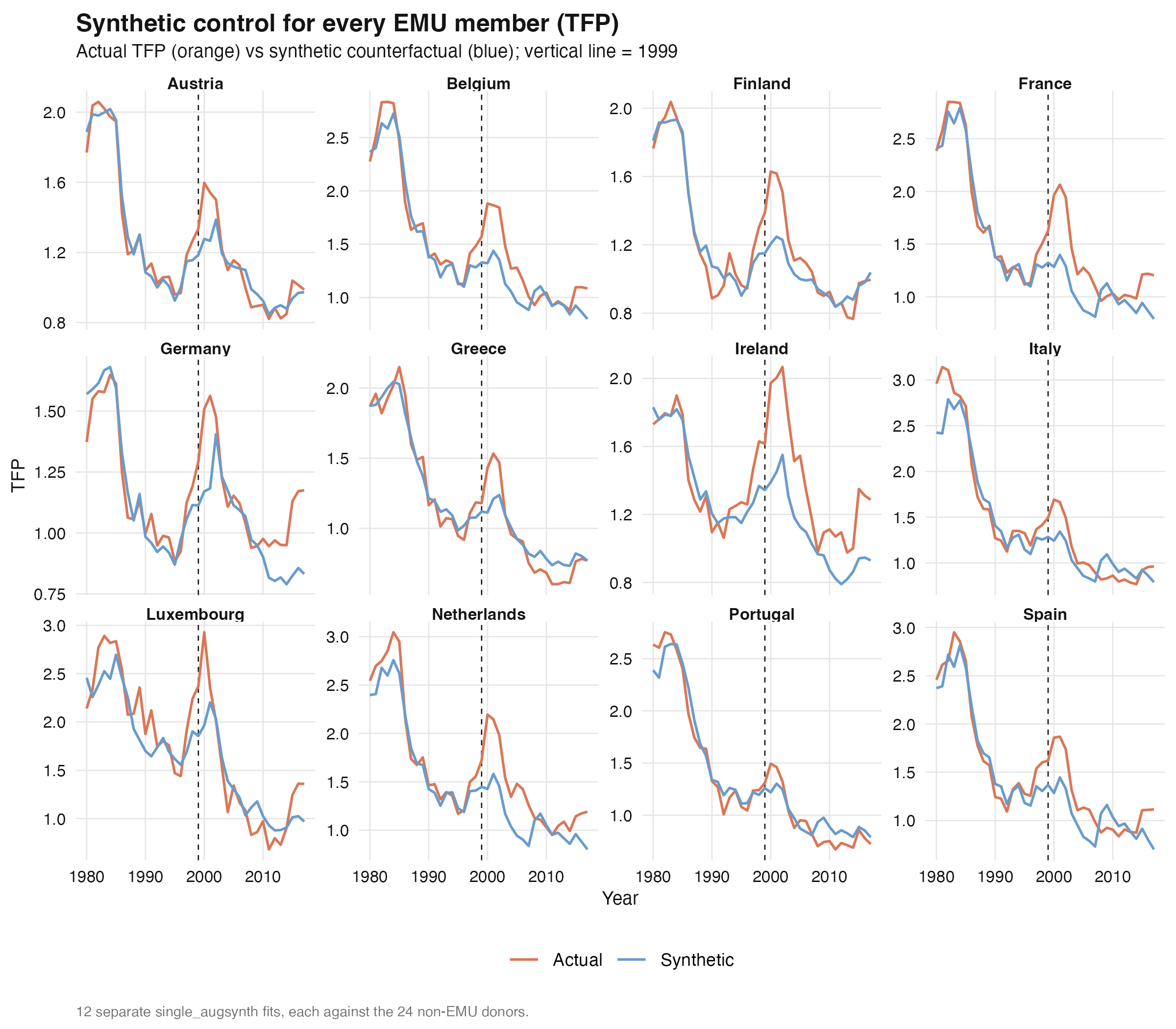
Fitting each member separately (twelve single_augsynth runs against the 24 donors) lets us see the heterogeneity behind the average. Most members run above their synthetic counterfactuals after 1999; Greece and Portugal converge to or fall below theirs after the crisis.

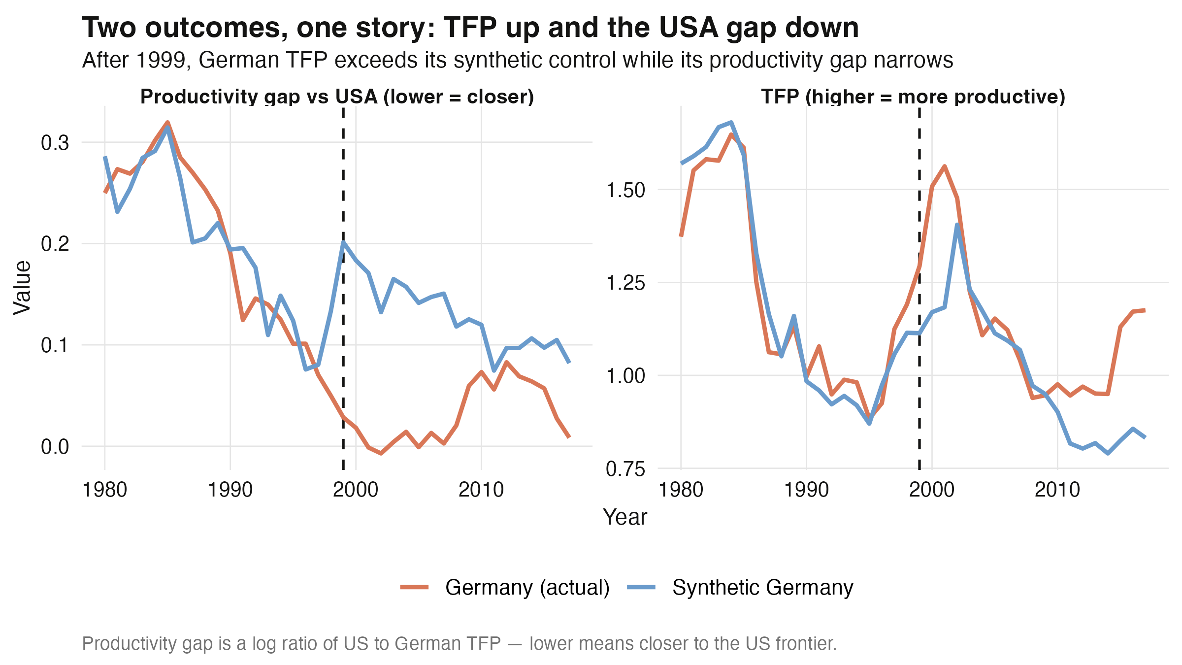
14. Two outcomes at once: augsynth_multiout on Germany

The euro should, in principle, move both German TFP and its productivity gap versus the USA. We estimate them jointly.

ger_mo <- augsynth_multiout(tfp + prod_gap ~ trt99, country, year, t_int = 1999,
                            germany_plus_donors, progfunc = "None", scm = TRUE,
                            combine_method = "concat")
summary(ger_mo)$average_att

   Outcome   Estimate   p_val
1      tfp     +0.116    0.603
2 prod_gap     -0.151    0.603

The two point estimates tell one coherent story: after the euro, German TFP rises (+0.116) and its productivity gap versus the USA narrows (−0.151, where a fall means catching up to the frontier). A single synthetic Germany, balanced on both series, supports both directions at once. But honesty requires the p-value: at 0.603 for each outcome, neither is statistically significant. The joint multi-outcome test is more demanding than the single-TFP conformal test (which was borderline at p = 0.027), and on one country’s real data the signal is not strong enough to clear it. The suggestive, coherent directions are worth reporting — as long as we do not overstate them as established.

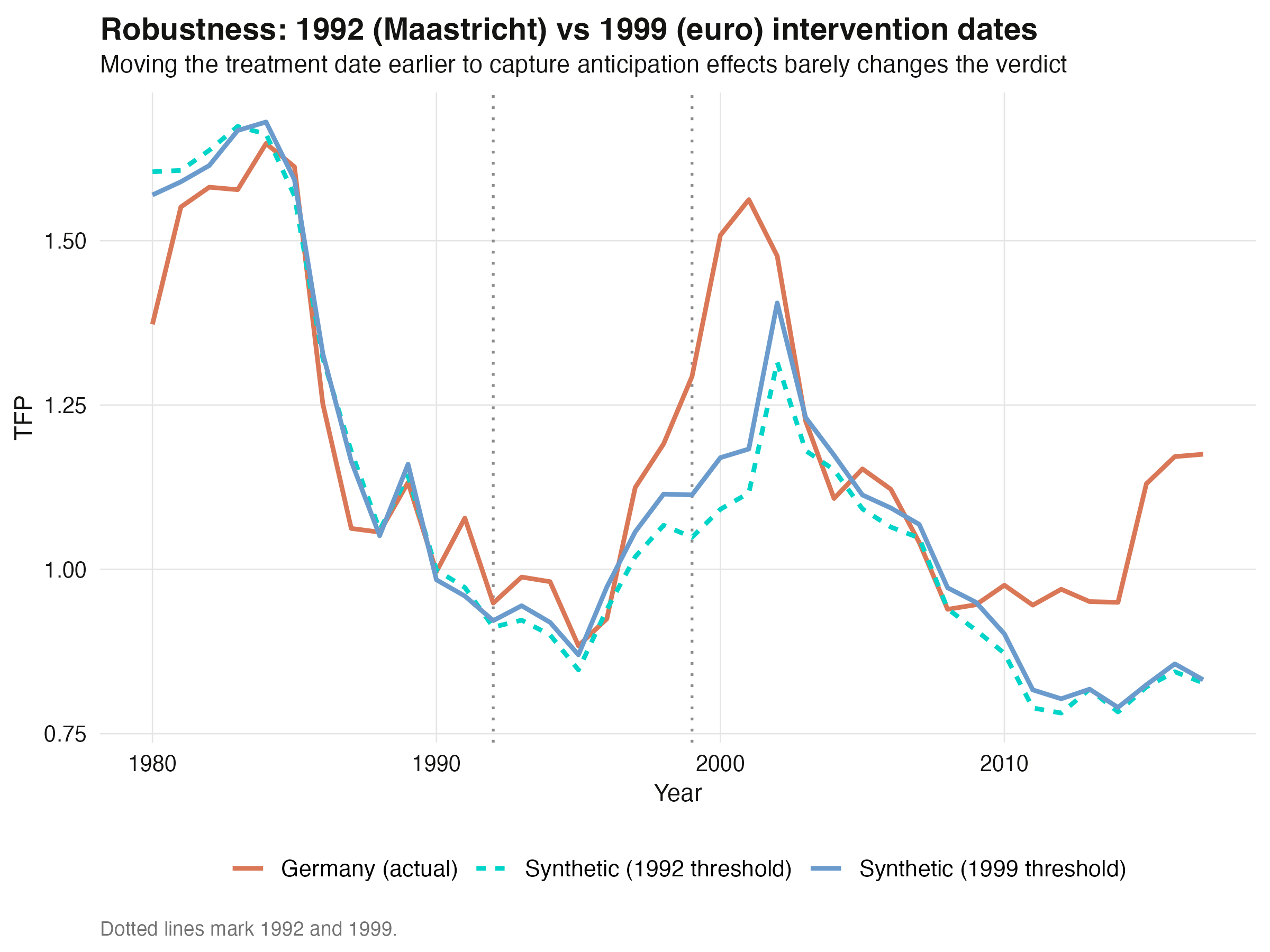
15. Robustness: the 1992 Maastricht threshold

Papaioannou notes that markets may have anticipated the euro from the 1992 Maastricht Treaty, not just the 1999 launch. We rerun Germany with the earlier threshold using the trt92 indicator.

ger_92 <- augsynth(tfp ~ trt92 | hum_cap + inv_share + ec_freed + patents + agricult,
                   country, year, germany_plus_donors, t_int = 1992,
                   progfunc = "None", scm = TRUE)

Germany avg ATT — 1999 spec: +0.133 | 1992 spec: +0.138

Moving the intervention date back seven years barely changes the estimate (+0.138 vs +0.133). The verdict is robust to the anticipation question, which strengthens the causal reading: whether we date the treatment at the treaty or the launch, synthetic Germany tells the same story.

16. Comparing to the paper

How close is our ASCM re-analysis to Papaioannou’s published numbers? The paper reports a percentage TFP “contribution” per country per period; we compute the analogous ASCM percentage effect and line them up for 2000–2007.

cor(comp$paper_2000_07, comp$ascm_2000_07, method = "spearman")

Correlation paper vs ASCM (2000-07 TFP % effect): Spearman 0.74 | Pearson 0.76
Both agree TFP rose for 12 of 12 members (ASCM).

The rank correlation between the paper’s numbers and ours is 0.74 (Pearson 0.76) — strong agreement given that augsynth uses a different estimator and donor-matching scheme than the paper’s classic SCM. Some countries land almost exactly on the 45-degree line (France: 42.7% vs the paper’s 43.6%; Netherlands: 44.0% vs 38.2%; Spain: 32.0% vs 26.9%), while a few diverge in magnitude (Germany and Ireland) but not in sign. Critically, the pattern replicates: large euro-era gains for France, the Netherlands, Belgium, Spain, and Ireland, and the post-crisis reversals for Greece (−12.4% in 2008–17) and Portugal (−14.3%) that the paper also reports.

We do not reproduce the paper’s numbers exactly, and we should not expect to: the estimators differ, and qualitative replication — same signs, same ranking, same dynamic story — is the right bar for a method comparison. By that bar, ASCM confirms the paper.

17. Discussion

Four threads tie Part 1 and Part 2 together.

Validate on truth, then trust on data. The single most useful habit this tutorial teaches is the order of operations: we confirmed that each augsynth function recovers a known effect on simulated data (errors under 5% for the well-fit units) before turning it loose on the euro question. When the EMU results then showed sensible signs and a clean pre-period, we had earned the right to believe them. A causal estimate you cannot first reproduce on simulated ground truth is a leap of faith.

Augmentation is insurance, not a free lunch. For well-fit units — C01–C04, and Germany — plain SCM and Ridge-ASCM agreed to the second decimal, and the Ridge penalty quietly switched itself off. The augmentation mattered exactly once: for C05, sitting outside the donor hull, where plain SCM got the sign wrong and Ridge-ASCM rescued it (mean error 0.737 → 0.128). The lesson is to read the pre-treatment imbalance every time and lean on augmentation only when the fit demands it.

Inference is a choice, and the choices can disagree. A point estimate is not a finding. On the simulated panel the pooled effect was significant under the jackknife but not under the wild bootstrap; on real German TFP the conformal p-value (0.027) and the jackknife+ interval (which included zero) split at the margin; the pooled euro effect and the joint multi-outcome test were honestly null. We reported the simulated headlines as significant (we injected them) and the borderline and null real-data results as exactly that. Match the inference tool to the estimator, report when methods disagree, and never let a near-zero estimate masquerade as a result.

Averages hide dynamics in multi-country work. The pooled multisynth effect on euro TFP was a forgettable −0.016 on average, yet the path revealed a +0.39 early bump erased by the 2008–2014 crisis. Two caveats travel with multisynth here: the EMU design is simultaneous (so the staggered features are demonstrated only on simulated data), and the pooled average is in raw TFP units, which mixes countries of very different productivity levels — making the per-country percentage effects the quantity truly comparable to the paper. Honest multi-country reporting means showing the path and the per-unit spread, not just the headline number.

18. Summary and next steps

• The Augmented Synthetic Control Method generalizes classic SCM with an outcome-model bias correction that is doubly robust: it helps when the pre-treatment fit is poor and does no harm when it is good.
• augsynth exposes three entry points: single_augsynth (one unit), multisynth (many units, staggered, pooled + per-unit), and augsynth_multiout (one unit, many outcomes). The top-level augsynth() dispatches to the right one.
• On simulated data with a known effect, all three recovered the truth closely and significantly (single +6.241 vs +6.250, jackknife+ [6.00, 6.51]; pooled multisynth +3.222 vs 3.155, jackknife [0.69, 5.75]; multiout +6.54 and +3.53, both conformal p < 0.001), and the suitability test showed Ridge-ASCM correcting a sign error that plain SCM could not — a wrong and non-significant estimate for C05.
• Inference is matched to the estimator — jackknife+ and conformal for a single unit, jackknife and the conservative wild bootstrap for multisynth, conformal p-values for multiple outcomes — and the methods can disagree. We reported significance honestly, including the borderline (Germany) and null (pooled euro, joint Germany) real-data cases.
• On the real EMU panel, ASCM qualitatively replicated Papaioannou (2021): a positive early TFP effect for most members (rank correlation 0.74 with the paper), Germany up and its US productivity gap narrowing, Greece and Portugal turning negative after the crisis, and robustness to the 1992-vs-1999 dating.

Where to go next: swap progfunc = "ridge" for other prognostic models ("gsyn", "mcp"); add covariate balancing after the | in the formula; explore in-time and in-space placebo tests for inference; or read the staggered-adoption theory in Ben-Michael, Feller, and Rothstein’s companion paper. The reusable synthetic_panel_multicountry.csv is a ready-made sandbox for any of these.

19. Exercises

1. Swap the outcome. Rerun the per-country EMU fits with prod_gap as the primary outcome instead of tfp. Does the productivity-gap story agree with the TFP story?
2. Stress the donor pool. Drop the single highest-weight donor from synthetic Germany and refit. How sensitive is the ATT to one donor?
3. Tune the pooling. Refit the simulated multisynth with nu = 0 (fully separate) and nu = 1 (fully pooled). How do the per-unit estimates and their confidence bands change?
4. Recover the negative. Using only synthetic_panel_multicountry.csv, reproduce C05’s negative effect with single_augsynth and explain why plain SCM fails.
5. Combine differently. In augsynth_multiout, switch combine_method = "avg" to "concat" and compare the two-outcome estimates. When might each be preferable?
6. Make inference disagree. For the simulated pooled multisynth effect, compute both inf_type = "jackknife" and inf_type = "bootstrap" intervals. Then shrink the panel (drop donors or pre-periods) and watch how each interval responds. Which one flips first, and why?

20. References

• Abadie, A., Diamond, A., & Hainmueller, J. (2010). Synthetic Control Methods for Comparative Case Studies. Journal of the American Statistical Association, 105(490), 493–505.
• Ben-Michael, E., Feller, A., & Rothstein, J. (2021). The Augmented Synthetic Control Method. Journal of the American Statistical Association, 116(536), 1415–1427.
• Ben-Michael, E., Feller, A., & Rothstein, J. (2022). Synthetic Controls with Staggered Adoption. Journal of the Royal Statistical Society: Series B, 84(2), 351–381.
• Papaioannou, S. K. (2021). European monetary integration, TFP and productivity convergence. Economics Letters, 199, 109696.
• augsynth package: https://github.com/ebenmichael/augsynth
• Feenstra, R. C., Inklaar, R., & Timmer, M. P. (2015). The Next Generation of the Penn World Table. American Economic Review, 105(10), 3150–3182.