Taming Model Uncertainty in the EKC

BMA and Double-Selection LASSO with panel data, graded against a known answer key

−7.139BMA recovers GDP coefficient · true −7.100

6 / 8true predictors flagged · zero false positives

2–3×bias when fixed effects are dropped

Carlos Mendez

Nagoya University (GSID)

July 8, 2026

The Tension

Act I

With 12 candidate controls, there are 4,096 ways to test the EKC — which one do you trust?

Does pollution fall as countries get rich? Testing the inverted-N Environmental Kuznets Curve needs a cubic in GDP — and a choice of controls.

With 12 candidates, \(2^{12} = 4{,}096\) regressions are possible. Picking one is a hidden assumption.

This is the model-uncertainty problem. The EKC is the substantive object — log CO2 per capita as a cubic function of log GDP, producing the inverted-N shape (fall, rise, fall). But beyond GDP, many controls might matter. Choosing a single specification is an unstated, consequential assumption. Two principled fixes: Bayesian model averaging and post-double-selection LASSO.

The GDP coefficient moves with the controls you choose

Coefficient	Sparse FE	Kitchen-sink FE	True DGP
\(\beta_1\) (GDP)	−7.498	−7.131	−7.100
\(\beta_2\) (GDP\(^2\))	0.849	0.806	0.810
\(\beta_3\) (GDP\(^3\))	−0.031	−0.030	−0.030

Same data, same fixed effects — the linear term swings from −7.498 to −7.131 just by adding controls.

Both standard specifications get the inverted-N sign pattern right (β1<0, β2>0, β3<0), but the magnitudes shift. Kitchen-sink is closer to the truth because the sparse model omits true controls and that biases it. But which of the 12 actually belong? Standard FE can’t tell you — it just hands you whichever model you chose.

A synthetic panel with an answer key lets us grade every method

Synthetic CO2 vs income: 80 countries, 1995–2014, N = 1,600. The cloud bends — the inverted-N shape the methods must recover.

The trick that makes this tutorial work: synthetic data with a known data-generating process. We designed it so that 5 controls truly affect CO2 and 7 are pure noise, with the true coefficients written down in advance. That turns “did the method work?” from a guess into an exam we can grade. Inspired by Gravina and Lanzafame (2025) but fully synthetic.

Where we’re going

• The lab: an 80-country, 20-year panel with a 5-true / 7-noise answer key
• Standard FE exposes the model-uncertainty problem
• BMA — average over 4,096 models, score each variable with a PIP
• Double-Selection LASSO — select controls twice, then run OLS
• The verdict: both work, but only with fixed effects in place

The Investigation

Act II

The lab: 80 countries × 20 years, 5 true controls hidden among 7 decoys

True predictors (5)

• fossil_fuel (+0.015)
• renewable (−0.010)
• urban (+0.007)
• democracy (−0.005)
• industry (+0.010)

Noise (7 decoys)

• globalization, services, trade, credit — correlated with GDP
• pop_density, corruption, fdi

Four decoys are deliberately correlated with GDP — they will look “significant” by piggybacking on GDP’s real effect.

N = 1,600 (80 countries, 20 years). The outcome is generated from a cubic EKC with country and year fixed effects plus the 5 true controls. The hard part: four noise variables are correlated with GDP, so a naive regression flags them as significant. The job of BMA and DSL is to see through that correlation and keep only the 5 true controls.

The model uncertainty we are fighting, written as one equation

\[\ln(\text{CO2})_{it} = \beta_1 \ln G_{it} + \beta_2 (\ln G_{it})^2 + \beta_3 (\ln G_{it})^3 + \mathbf{X}_{it}^{\text{true}}\boldsymbol{\gamma} + \alpha_i + \delta_t + \varepsilon_{it}\]

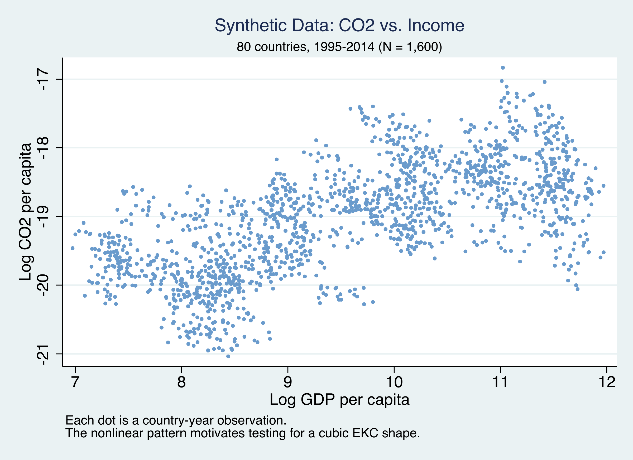
A cubic in log GDP \(G\) gives the inverted-N; \(\alpha_i\) and \(\delta_t\) absorb country and year heterogeneity; \(\mathbf{X}^{\text{true}}\) is the 5 controls we must rediscover.

This is the true DGP. The inverted-N needs β1<0, β2>0, β3<0, and we built it with exactly that pattern (−7.1, 0.81, −0.03). Country fixed effects α_i and year effects δ_t soak up unobserved heterogeneity — keep this in mind, because dropping them later breaks everything. The exam: can BMA and DSL recover both the cubic shape and the 5 true controls?

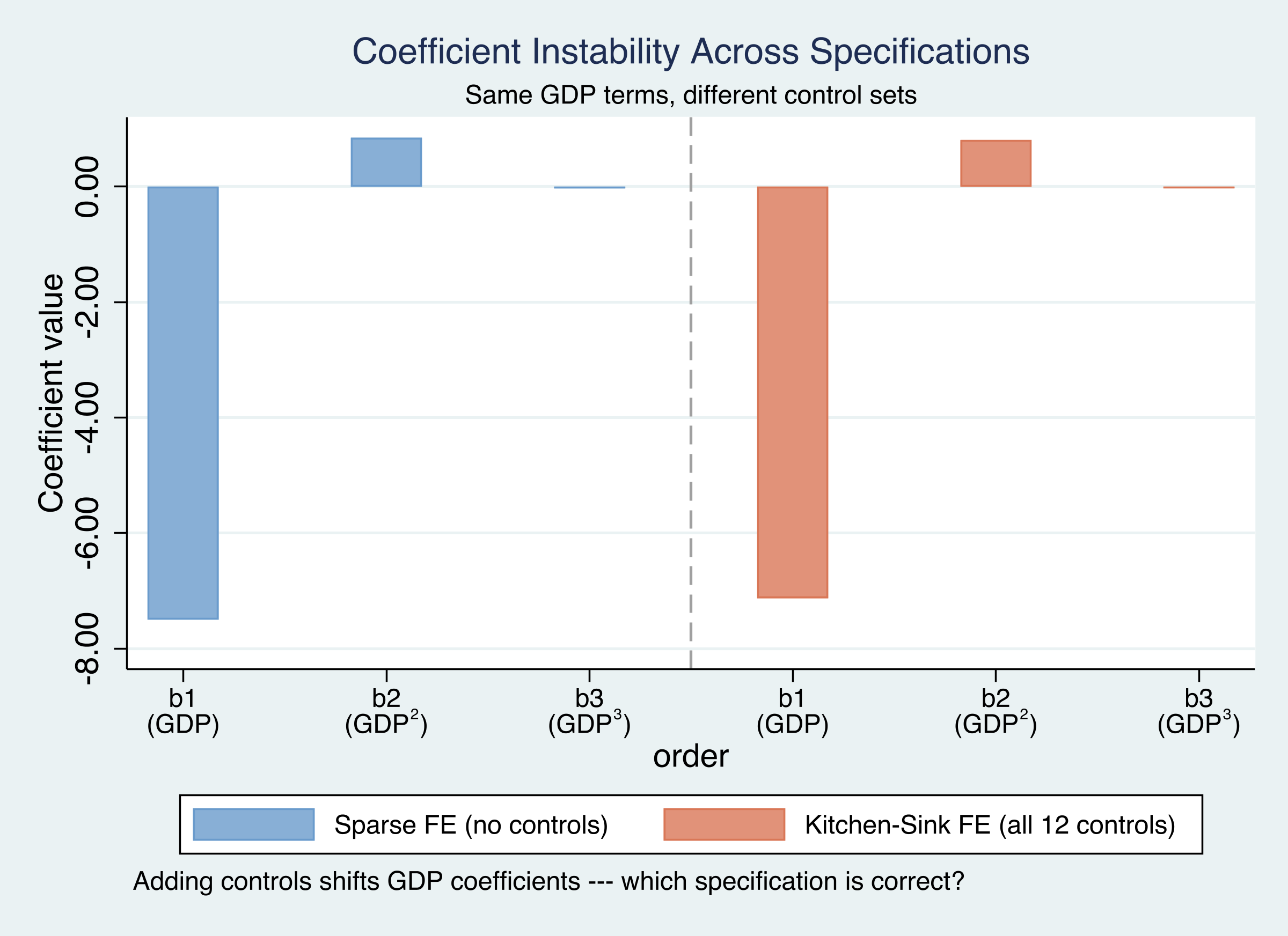
Adding all 12 controls shifts the GDP coefficient — yet still won’t say which controls belong

GDP polynomial coefficients shift between the sparse and kitchen-sink fixed effects specifications — the visible signature of model uncertainty.

The kitchen-sink regression (all 12 controls) gets the three strong predictors right — fossil fuel, industry, urban are significant — and most noise variables are insignificant. But democracy’s estimate (−0.0003, p=0.97) is nowhere near its true −0.005: weak signals are hard even with the correct model. The coefficients shift enough to move the turning points by ~$2,000. Standard FE leaves us guessing.

BMA averages over all 4,096 models and weights each by how well it fits

\[P(M_k \mid \text{data}) = \frac{P(\text{data} \mid M_k)\, P(M_k)}{\sum_{l} P(\text{data} \mid M_l)\, P(M_l)}\]

Each model’s weight is its fit (marginal likelihood) times its prior. Better-fitting, parsimonious models earn more weight — BMA’s built-in Occam’s razor.

Instead of betting on one horse, BMA spreads bets across the whole field.

The marginal likelihood integrates over all coefficient values, so a model with many parameters spreads its prior thin and only recovers that probability if the data strongly support the extra dimensions. That is why BMA automatically penalizes complexity. With these weights in hand we can do two things: average coefficients, and score each variable.

The PIP is a democratic vote: what share of good models keep a variable?

\[\text{PIP}_j = \sum_{k:\, x_j \in M_k} P(M_k \mid \text{data})\]

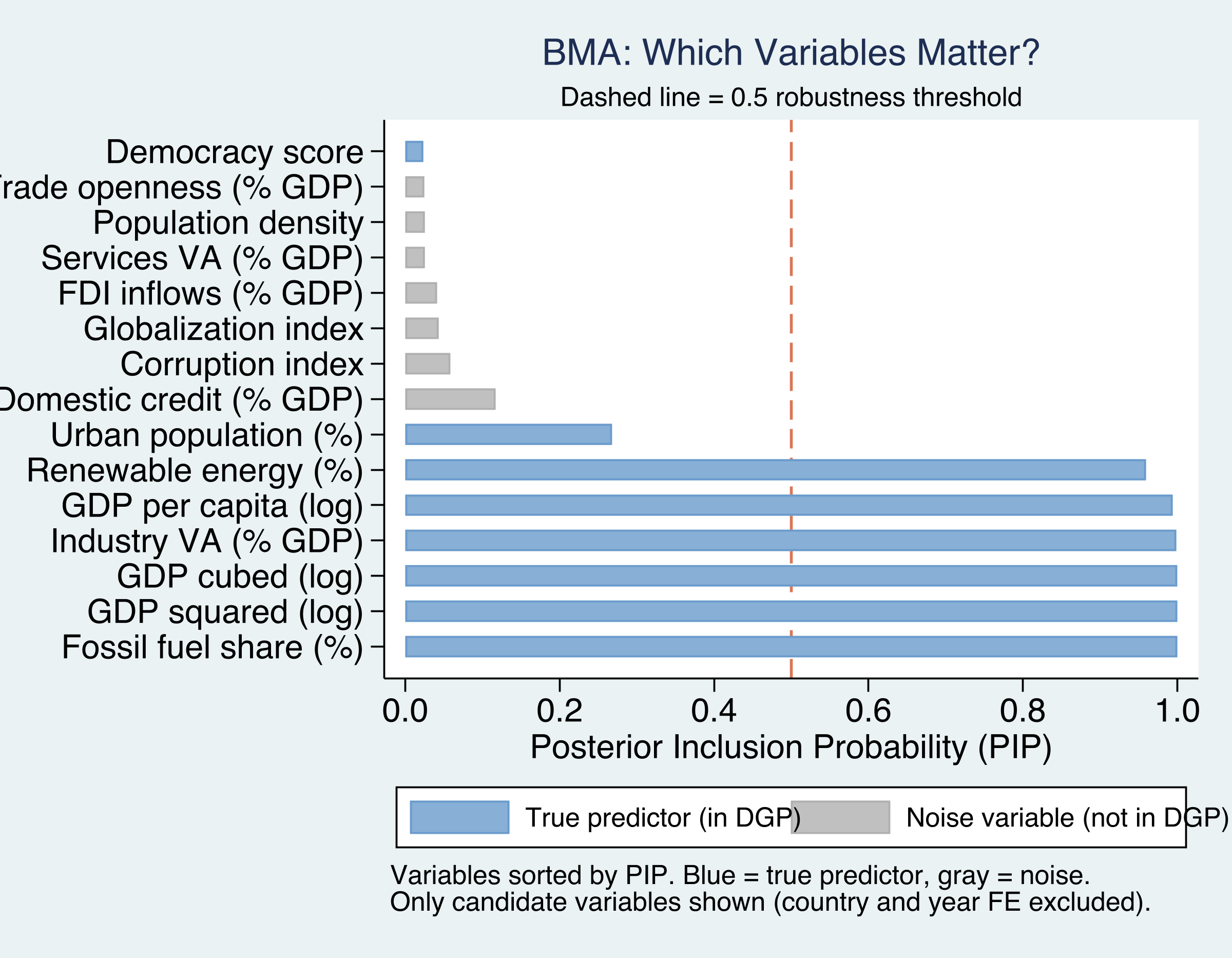
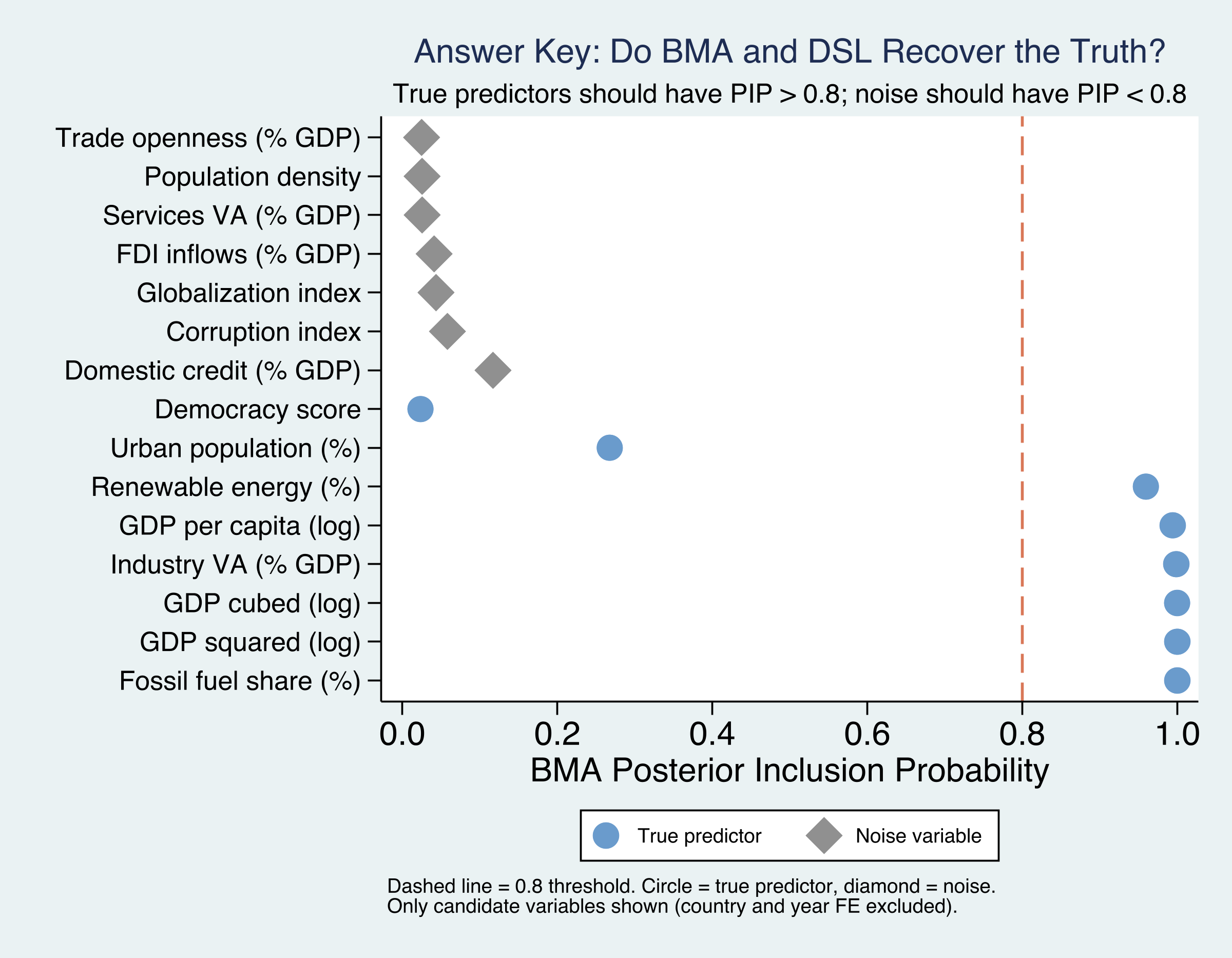
A variable in every high-probability model has \(\text{PIP} \to 1\); one only in long-shot models stays near 0. We treat \(\text{PIP} \geq 0.80\) as “robust.”

PIP sums the posterior weight of every model that contains the variable — Raftery’s thresholds: ≥0.99 decisive, 0.95–0.99 very strong, 0.80–0.95 strong/robust, below 0.50 weak. 0.80 is the standard applied cutoff. The BMA posterior mean shrinks each coefficient toward zero in proportion to the evidence against inclusion, so a PIP of 0.5 roughly halves the conditional estimate. PIP is the signature output we grade against the answer key.

Six lines of Stata run BMA with fixed effects always in the model

bmaregress $outcome $gdp_vars $controls ///
    ($fe, always), ///
    mprior(uniform) groupfv gprior(uip) ///
    mcmcsize(50000) rseed(9988) inputorder pipcutoff(0.8)

($fe, always) forces country and year FE into every model; groupfv moves the 80 country dummies as one package, not 80 independent choices.

Uniform model prior = every model equally likely a priori; UIP = unit-information g-prior, relatively uninformative. mcmcsize draws 50,000 models via MC³; rseed fixes reproducibility. Without groupfv, i.country_id would be 80 separate selection choices — a 2^80 model space, meaningless. With it, the dummies enter or leave as a roster. pipcutoff(0.8) is a display threshold only.

BMA recovers the GDP coefficient almost exactly — −7.139 vs true −7.100

−7.139

BMA posterior mean on \(\beta_1\) · true DGP value −7.100; cubic term −0.030 matches the truth exactly

The three GDP terms come back at −7.139, 0.808, −0.030 against the truth −7.100, 0.810, −0.030 — within about 1% each, and the cubic term is exact to three decimals. This is meaningfully closer than the sparse FE (−7.498). BMA averaged over 163 sampled models (of 4,096) with sampling correlation 0.9997, concentrating on the high-probability region rather than visiting every model.

BMA flags 6 of 8 true predictors and zero noise — the answer key confirmed

PIPs for all 15 variables: true predictors (steel blue) clear the 0.80 line; all 7 noise variables (gray) sit near zero.

Top of the chart, near PIP 1.0: the three GDP terms, fossil fuel (1.000), industry (0.999), renewable (0.959) — six of the eight true predictors flagged robust. Bottom, near zero: all seven noise variables, correctly rejected. Zero false positives. The only misses are urban (PIP ≈ 0.27) and democracy (≈ 0.02), whose true coefficients (+0.007, −0.005) are simply too small to detect at this sample size — an honest limitation, not a failure.

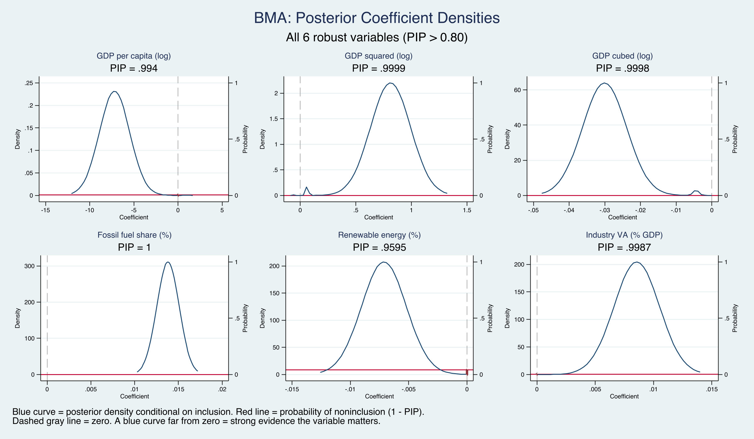
The posterior densities sit far from zero — strong evidence for all six robust variables

Posterior coefficient densities for the six PIP > 0.80 variables. Top row: GDP linear, squared, cubic. Bottom: fossil fuel, renewable, industry. All concentrated away from zero.

Each blue curve is the density conditional on inclusion; the flat red line is the probability of non-inclusion (1 − PIP). Near-zero red line plus a blue curve far from zero = strong evidence. The GDP terms center on −7.1, +0.81, −0.030 (the truth); the controls on +0.014, −0.007, +0.009. Renewable’s −0.007 is slightly attenuated from its true −0.010 — BMA shrinkage, because its PIP is below 1.0.

DSL takes a different road: select controls twice, then run a clean OLS

\[\hat{S} = \hat{S}_Y \cup \hat{S}_{D_1} \cup \hat{S}_{D_2} \cup \hat{S}_{D_3}, \qquad \hat{\boldsymbol{\beta}}^{\text{LASSO}} = \arg\min_{\boldsymbol{\beta}}\ \tfrac{1}{2N}\textstyle\sum_i (y_i - \mathbf{x}_i'\boldsymbol{\beta})^2 + \lambda\sum_j |\beta_j|\]

LASSO on the outcome (\(\hat S_Y\)) and on each GDP term (\(\hat S_{D_k}\)); the union is the safety net; then OLS on that union.

The second selection catches a confounder the outcome-LASSO would miss — that is the “double.”

Belloni, Chernozhukov & Hansen (2014). The L1 penalty’s sharp corner at zero forces weak coefficients to exactly zero — that is what makes LASSO a selector, unlike Ridge. The union is the key insight: a control that predicts the treatment but only weakly predicts the outcome could be dropped by a single outcome-LASSO and bias the GDP coefficient. The d-LASSO catches it. dsregress chooses λ by a plugin formula, no cross-validation.

With fixed effects, DSL gives fast, valid estimates — −7.433 in seconds

Coefficient	DSL (FE)	True DGP	Significant?
\(\beta_1\) (GDP)	−7.433	−7.100	yes
\(\beta_2\) (GDP\(^2\))	0.840	0.810	yes
\(\beta_3\) (GDP\(^3\))	−0.031	−0.030	yes

Cluster-robust SEs, four internal LASSOs, union, then OLS — all in seconds. Wald \(\chi^2 = 53.15\), \(p < 0.001\).

DSL lands between the sparse and kitchen-sink FE, close to BMA. Why not closer to the truth? In this panel, 99 of 112 candidates are FE dummies; LASSO retains nearly all of them (102 of 112) and has little room to discriminate among the 12 controls of interest. So the final OLS sits near the kitchen-sink. To see LASSO’s selection power unleashed, you have to remove the FE — which we do next, with a warning.

Strip the fixed effects and the GDP coefficient explodes to −21.26

−21.26

Pooled BMA \(\beta_1\) (no FE) · 3× the true −7.100; pooled DSL agrees at −22.03

Treat the panel as a pooled cross-section — no country or year effects — and both methods inflate the GDP coefficient 2–3x. Pooled BMA gives −21.26, pooled DSL −22.03. The fact that a Bayesian and a frequentist method agree so closely on the WRONG answer is the tell: the bias is not about variable selection, it is the omitted fixed effects. The GDP terms absorb persistent cross-country differences in emissions levels.

Worse, pooled BMA hands robust status to 5 noise variables

With fixed effects

• 6 variables clear PIP \(\geq 0.80\)
• all 7 noise → PIP \(\approx 0\)
• zero false positives
• intervals cover the truth

Pooled (no FE)

• 12 of 15 clear PIP \(\geq 0.80\)
• services, credit, pop. density → PIP = 1.000
• 5 false positives
• intervals miss the truth, all 3 terms

This is the sharpest lesson in the deck. Without FE, the noise variables are correlated with the omitted country effects, and BMA reads those spurious correlations as genuine predictive power. PIP thresholds are only meaningful when the model set is correctly specified. The pooled credible intervals are actually narrower than the FE ones — false precision from a misspecified model, the worst case.

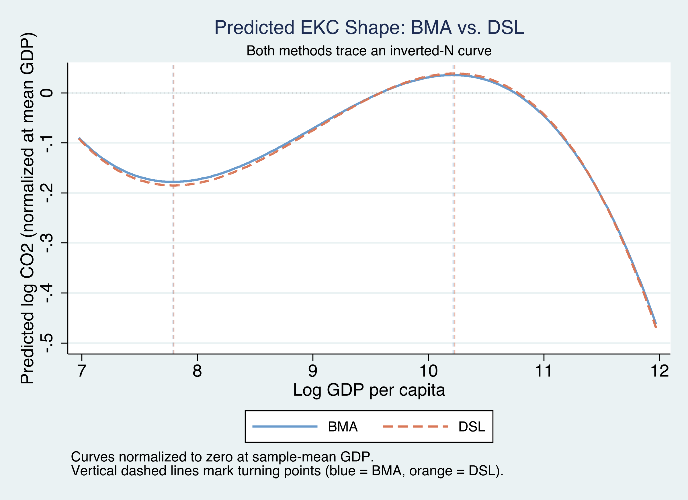
Both curves trace the same inverted-N — BMA and DSL agree on the shape

Predicted EKC curves (normalized at mean GDP): BMA (solid blue) and DSL (dashed orange) are nearly indistinguishable, with closely aligned turning points.

Normalizing both curves to zero at the sample-mean GDP makes the shape pop. CO2 falls at very low income, rises through industrialization, falls again at high income — the inverted-N. The two methods, built on entirely different logic (Bayesian averaging vs frequentist selection), land on essentially the same curve. When a Bayesian and a frequentist method agree on the correctly specified model, the finding is robust.

Does machine selection make this causal? No — it disciplines, it does not identify

Objection. “BMA and LASSO pick controls automatically — surely that delivers the causal effect of income on emissions.”

Response. No. These are model-uncertainty tools, not identification tools. They tame which controls enter and report honest robustness (PIPs, valid SEs). Identifying a causal EKC still needs the usual assumptions — and the synthetic answer key grades recovery of a known DGP, not a real-world causal claim.

Steelman, don’t strawman. BMA and DSL solve “which of these candidate controls belong?” and “how robust is each?” They do not manufacture identification — endogeneity (e.g. via 2SLS-BMA in Gravina & Lanzafame), reverse causality, and omitted confounders outside the candidate set remain the analyst’s job. This deck demonstrates accurate variable selection against ground truth, framed as model averaging and robustness, not a causal estimand.

The Resolution

Act III

The verdict: 6 of 8 true predictors recovered, zero false positives — with fixed effects

Answer key: BMA PIPs by ground truth. True predictors (blue circles) cluster above 0.80; noise variables (gray diamonds) cluster below.

BMA’s report card: of 8 true predictors (3 GDP terms + 5 controls), it flags 6 at PIP > 0.80 with zero false positives — only the two weak-signal misses (urban, democracy). DSL gives fast, valid cluster-robust estimates in seconds. Both recover the inverted-N. The synthetic answer key confirms both are doing their job, with the expected limitation that weak signals are genuinely hard to detect.

Choose the tool by the question — averaging vs fast valid inference

Use BMA when…

• the question is which variables robustly predict?
• you want PIPs + coefficient densities
• most accurate here: −7.139 vs −7.100
• cost: MCMC takes minutes

Use DSL when…

• you have a clear variable of interest + many controls
• you want fast, valid frequentist inference
• runs in seconds, cluster-robust SEs
• limited by FE-heavy candidate sets

Different questions, not better/worse. BMA’s wider credible intervals honestly account for model uncertainty by averaging across thousands of models; frequentist methods condition on one model and understate it. Best of all: run both. If a Bayesian and a frequentist method agree on sign, magnitude, and significance, the finding is unlikely to be an artifact of any single modeling choice — and disagreements flag where evidence is assumption-sensitive.

Tame model uncertainty with BMA or DSL — but absorb the fixed effects first.

The single takeaway. Both methods recover the inverted-N EKC and the true predictors — BMA’s −7.139 is the closest of all to the truth’s −7.100, with zero false positives. But strip the fixed effects and both inflate the GDP coefficient 2–3x and invent five robust noise variables. Method agreement is no substitute for correct specification: in panel data, absorb the unobserved heterogeneity before you average or select.