Beta and Sigma Convergence Across Countries

Are poor countries catching up? A convergence toolkit in Stata

0.36%/yrconvergence speed since 2000

190 yrhalf-life of the income gap

+91%rise in income dispersion

Carlos Mendez

Nagoya University (GSID)

June 11, 2026

The Tension

Act I

Are poor countries doomed to stay poor — or is the gap finally closing?

If poorer economies grow faster than richer ones, today’s vast income gaps close on their own.

For four decades the evidence said no: from 1960 to 2000 the rich pulled further ahead. So is convergence simply dead?

This is the oldest question in development economics. Convergence is the optimistic hypothesis — that the gap is self-correcting. The discouraging fact is that for most of the post-war era the data flatly rejected it: poor countries were not catching up, they were falling behind. The whole talk hangs on whether that verdict still holds.

Over six decades, where a country started told you nothing about how fast it grew

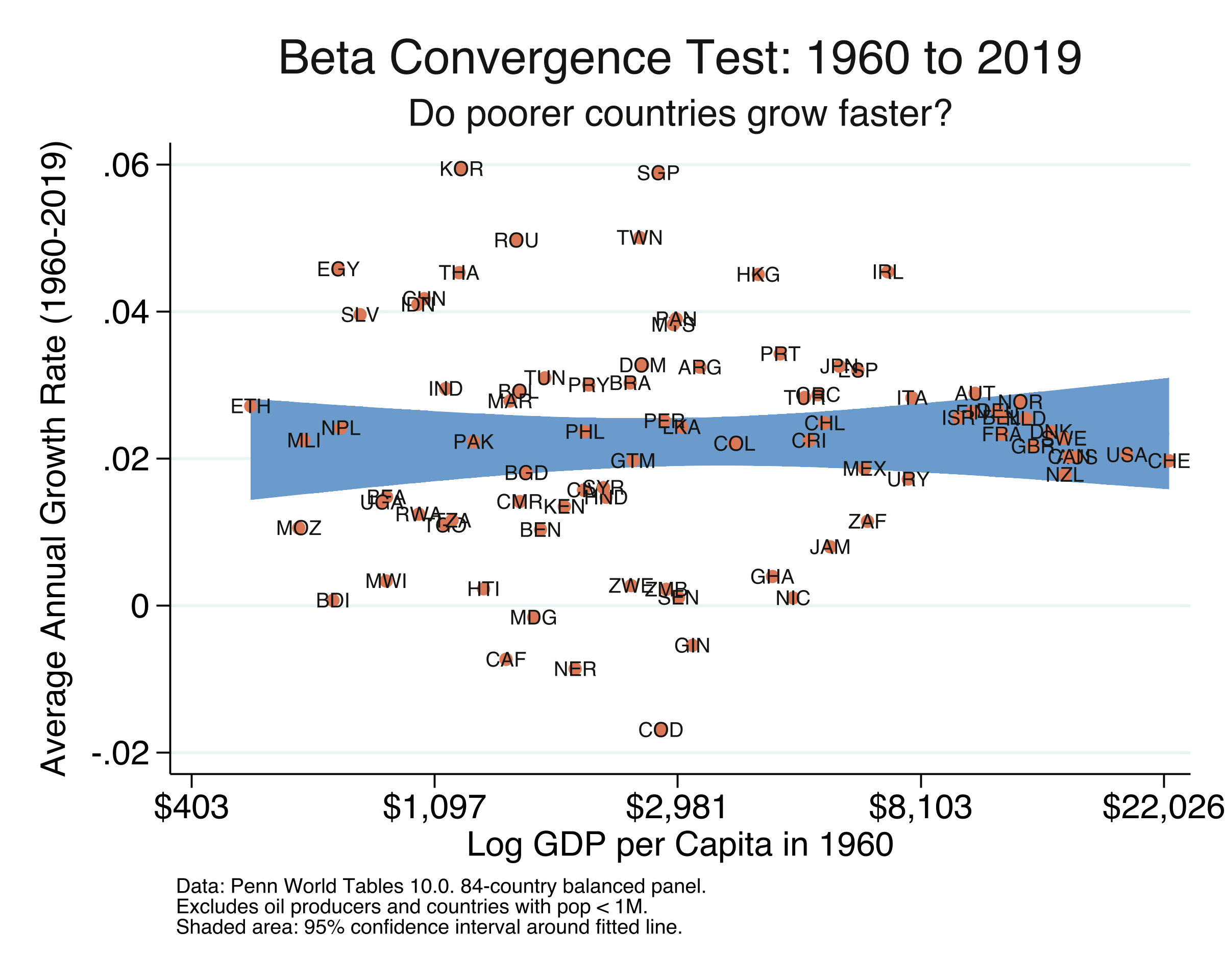
Annualized growth (1960–2019) versus log initial income. The fitted line is flat: starting income has essentially no predictive power.

This is the post’s first money chart — and a deliberate red herring. The OLS slope is 0.00057 (p = 0.661), R-squared 0.0013. Statistically indistinguishable from a flat line. The naive reading: six decades, no convergence, case closed. Plant that conclusion now; Act II will demolish it.

Two convergence ideas — and the surprise that one doesn’t guarantee the other

Beta convergence

• Do poor countries grow faster?
• A regression slope on initial income
• \(\lambda < 0 \Rightarrow\) catch-up

Sigma convergence

• Is the income spread shrinking?
• The variance of log income over time
• \(\sigma_t^2\) falling \(\Rightarrow\) narrowing

The twist this talk delivers: beta convergence can be real while the distribution still widens.

Keep these two straight throughout. Beta = a behavioural tendency (rear runners are faster). Sigma = an outcome (is the pack actually bunching?). Young, Higgins & Levy proved beta is necessary but not sufficient for sigma. The whole Act III payoff is that we observe exactly this gap.

Where we’re going

• The data: a balanced 84-country panel, 1960–2019
• Split at 2000 — a hidden structural break
• Turning an OLS slope into a speed and a half-life
• NLS: estimating that speed directly, and why it agrees
• Sigma convergence — and the 8-year lag that breaks the link

The Investigation

Act II

The lab: 84 countries, 60 years, one balanced panel from PWT 10.0

• Outcome — annualized growth of real GDP per capita (PPP)
• Predictor — log income in the start year
• Sample — 84 countries with data since 1960; oil producers and sub-1M-population states excluded

5,040 country-year rows. Balanced means the same 84 countries appear every year — so no composition effects.

Penn World Tables 10.0, expenditure-side real GDP at chained PPPs — comparable across price levels. Following Patel, Sandefur & Subramanian (2021) we drop oil economies (income is resource rent, not productive catch-up) and tiny states. Balancing the panel is the load-bearing design choice: it fixes N = 84 in every year, so the sigma series later can’t be contaminated by countries entering or leaving.

The regression is one line: growth on log initial income

\[g_i = \alpha + \lambda \cdot \ln(y_{i,0}) + \varepsilon_i\]

\(g_i\) is country \(i\)’s annualized growth; \(\ln(y_{i,0})\) is its log starting income. A negative \(\lambda\) means convergence — the poor grow faster.

This is unconditional (absolute) beta convergence: no controls for institutions, schooling, or savings. It’s the strong form of the hypothesis. The sign of one coefficient settles the direction; everything that follows refines its magnitude and stability.

Split at 2000 and the flat line shatters into two opposite eras

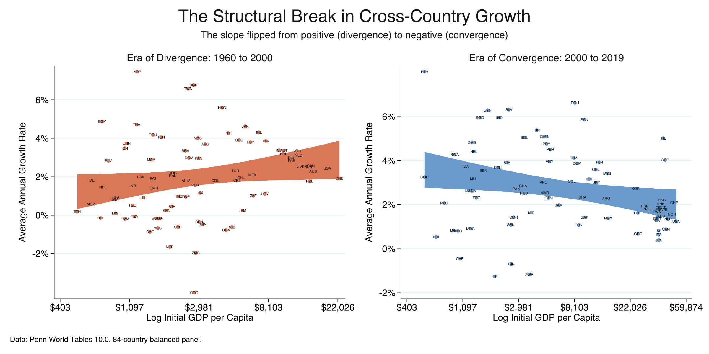
Era of divergence (1960–2000, orange) versus era of convergence (2000–2019, steel): the slope flips sign.

1960–2000: lambda = +0.00437 (p = 0.007) — richer countries grew faster, the gap widened. 2000–2019: lambda = -0.00352 (p = 0.019) — poorer countries now grow faster. The full-period slope averaged these two regimes into a null. This is the structural break Patel et al. call “the new era of unconditional convergence.”

Before 2000 the gap widened; after 2000 it began to close

Period	\(\lambda\)	p	Verdict
1960–2000	+0.00437	0.007	divergence
2000–2019	−0.00352	0.019	convergence

A total swing of 0.0079 — a complete reversal that the 60-year pooled regression silently averaged away.

A textbook reminder of why pooled estimates mislead: when the sign of a relationship flips mid-sample, the full-period coefficient can read as “nothing happened.” The story is the break. Chow tests, rolling windows, and a year-2000 dummy all locate it at the same place.

A slope isn’t a speed — convert \(\lambda\) into the structural \(\beta\)

\[\beta = \frac{-\ln(1 + \lambda s)}{s} \qquad\qquad \tau = \frac{\ln 2}{\beta}\]

\(\lambda\) depends on the window length \(s\); the Barro–Sala-i-Martin speed \(\beta\) does not. The half-life \(\tau\) is the years to close half the gap.

The raw OLS slope mixes the convergence speed with how long the window is, so it can’t be compared across periods. Barro & Sala-i-Martin (1992) show lambda = -(1 - exp(-beta·s))/s; invert it and you get beta as a function of lambda and s. Half-life is just the radioactive-decay formula — the most human-readable summary of beta.

Convergence since 2000 runs at 0.36% a year — five times slower than the benchmark

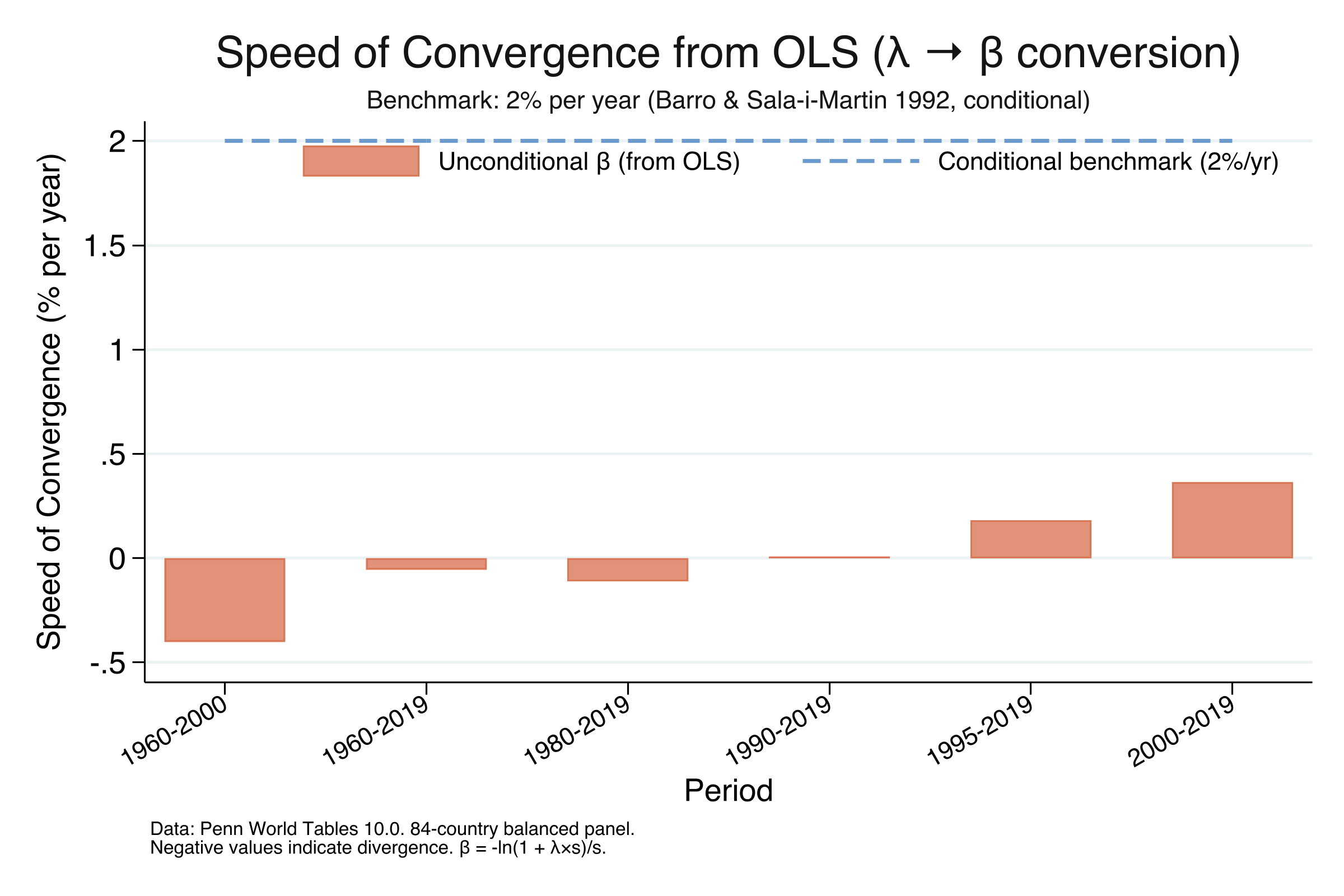
Speed of unconditional convergence (β) across six windows; dashed line = the classic 2% conditional benchmark.

Acceleration as the start year moves forward: 1960–2000 still divergence (beta = -0.0040), then 0.18% for 1995–2019, then 0.36% for 2000–2019. The dashed 2%/yr line is the conditional-convergence benchmark from the 1990s — what you get after controlling for human capital and institutions. Unconditional convergence is real but roughly five times weaker.

The number that should temper optimism: a 190-year half-life

190 years

to close half the income gap at the 2000–2019 speed (\(\beta = 0.00365\))

At this pace a country at one-tenth of US income would need nearly two centuries just to halve the distance — not to catch up, merely to close half the gap. The classic conditional benchmark is a 35-year half-life. Convergence exists, but it is glacial.

Why not estimate \(\beta\) directly? The trouble is it hides inside an exponential

\[\frac{1}{s}\ln\!\frac{y_{i,t+s}}{y_{i,t}} = \alpha - \frac{1 - e^{-\beta s}}{s}\,\ln(y_{i,t}) + \varepsilon_i\]

OLS needs parameters to enter linearly. Here \(\beta\) is trapped in \(e^{-\beta s}\) — so OLS can only recover the whole blob \(\lambda\), then we back out \(\beta\).

This motivates NLS. OLS estimates the bracketed expression as a single coefficient lambda; the structural beta must be extracted algebraically afterward. Nonlinear least squares minimises the same sum of squared residuals but allows the parameter to sit inside any function — so it can chase beta directly.

Stata’s nl estimates \(\beta\) in one line — start it at the 2% benchmark

local s = 19
nl (outcome = {b0=1} - (1 - exp(-1*{b1=0.02}*`s'))/`s' * initial_inc), vce(robust)

{b1=0.02} is \(\beta\) with the 2% benchmark as its starting guess; the iterative solver then minimises squared residuals.

nl puts the full nonlinear equation in parentheses and free parameters in curly braces with starting values. {b0} is the intercept, {b1} is beta. vce(robust) gives heteroskedasticity-robust SEs. The big payoff: the SE and p-value attach to beta itself — no delta method needed.

OLS-then-convert and direct NLS agree to seventeen decimal places

Period	OLS → \(\beta\)	NLS \(\beta\)	difference
2000–2019	+0.00365	+0.00365	\(10^{-17}\)
1995–2019	+0.00182	+0.00182	\(10^{-17}\)
1960–2000	−0.00402	−0.00402	\(10^{-16}\)

The Barro–Sala-i-Martin equation is a reparameterization of the linear model — so the two routes must coincide.

The differences are numerical noise, ~10^-17. Both minimise the same residual sum of squares; only the parameterization differs. So the choice is convenience, not correctness: OLS for speed and guaranteed convergence of the solver, NLS when you want inference on beta directly.

Watch convergence switch on: the rolling slope crosses zero around 1990

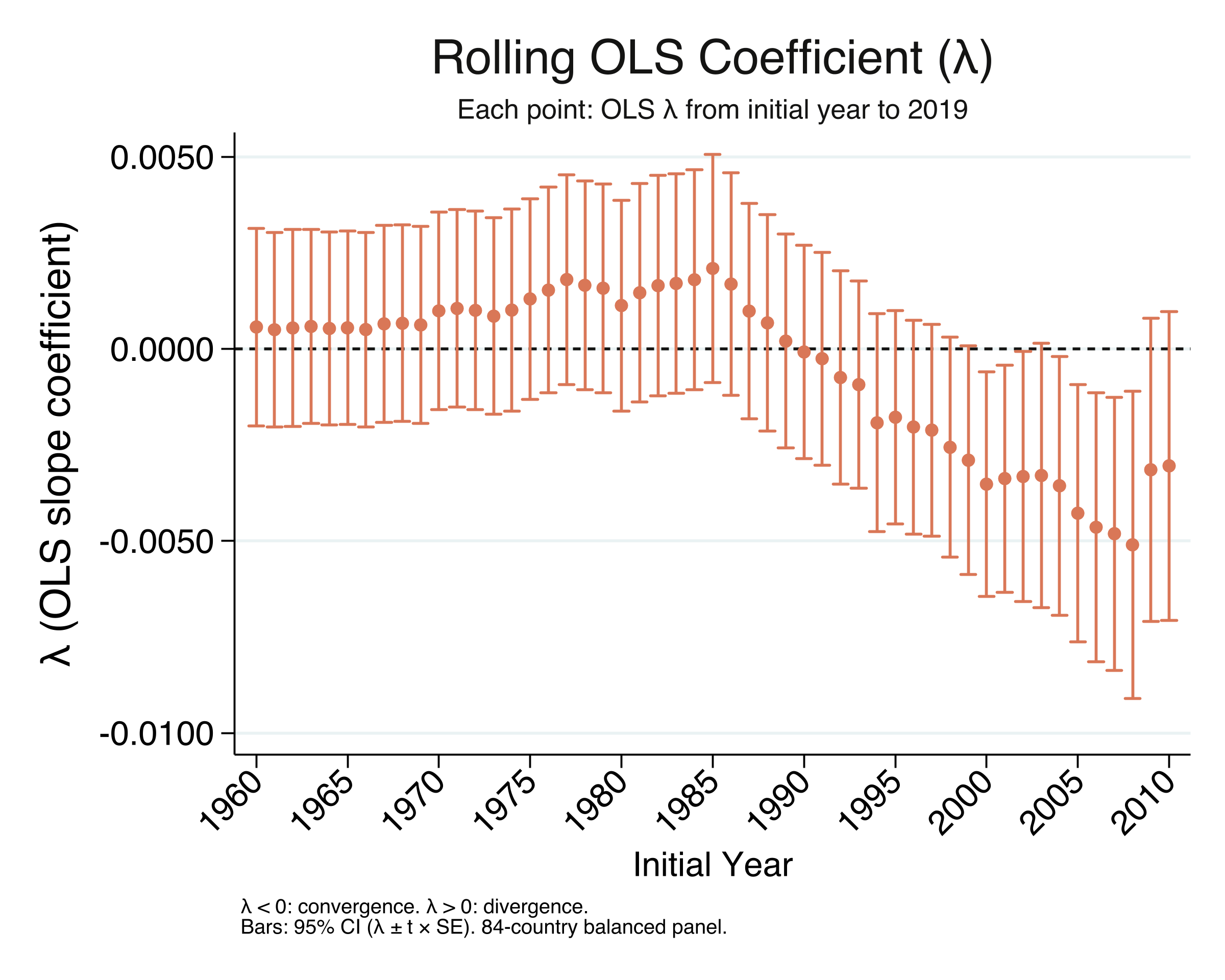
Rolling OLS \(\lambda\) from each start year to 2019, with 95% confidence intervals. Negative \(\lambda\) = convergence.

Each dot is a separate regression with the start year sliding from 1960 to 2010 and the end fixed at 2019. Positive (divergence) through the 1980s, crossing zero near 1990, solidly negative — and statistically distinguishable from zero — for start years from about 1998 on. Remember the sign flip: negative lambda but positive beta both mean convergence.

As \(\beta\), the same story peaks near 2005 then eases — the crisis footprint

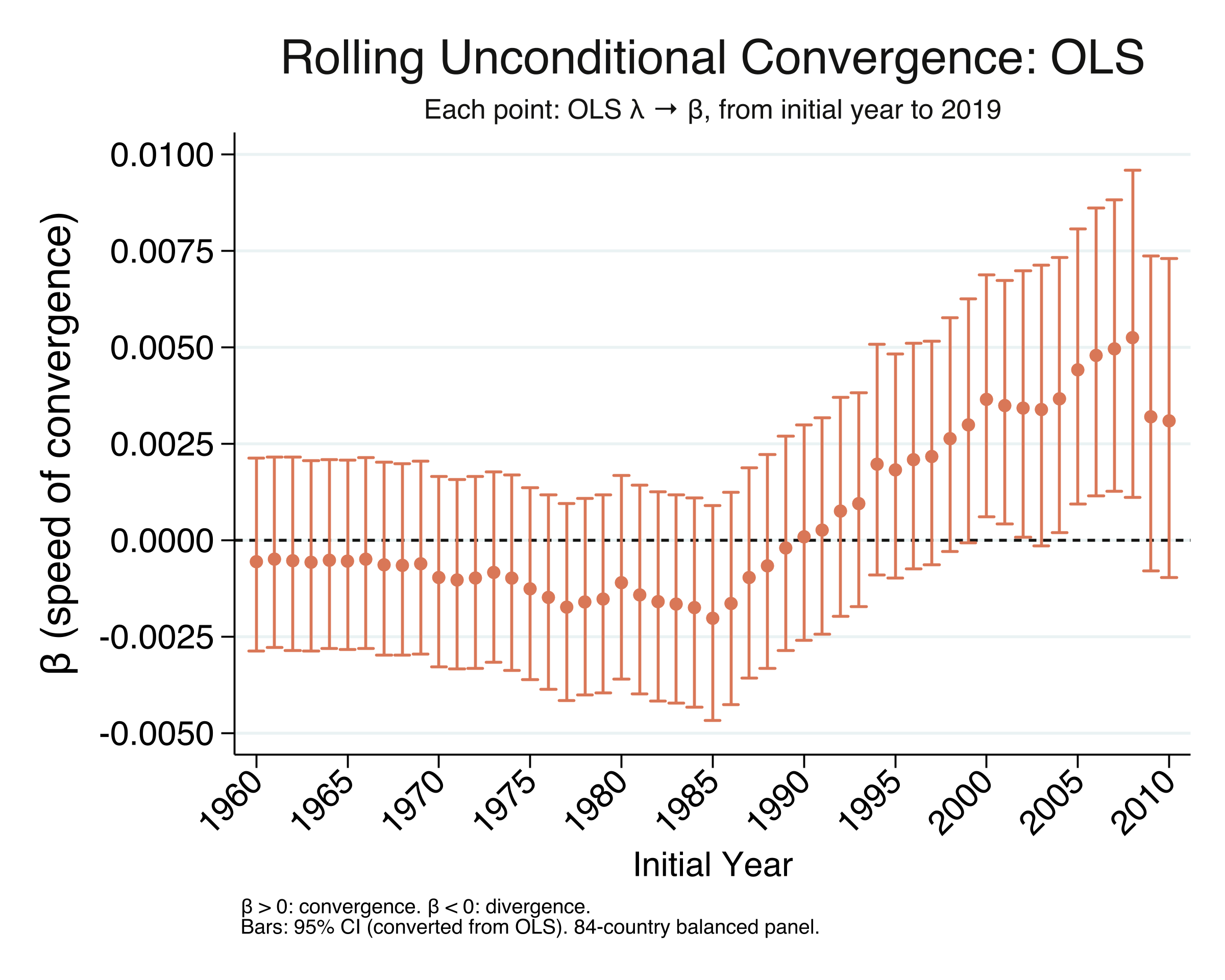
Rolling structural \(\beta\) (OLS conversion; NLS is identical) from each start year to 2019, with 95% CIs.

Beta climbs through the 1990s, crosses zero around 1990, peaks at 0.00441 (half-life 157 yr) for start year 2005, then pulls back to 0.00309 for 2009–2010 — plausibly the 2008 financial crisis. The NLS rolling figure is visually identical; only the CI construction differs (NLS straight from beta’s SE, OLS transformed from lambda’s with a bound-flip).

The Resolution

Act III

Beta convergence is real — yet the income spread grew by 91%

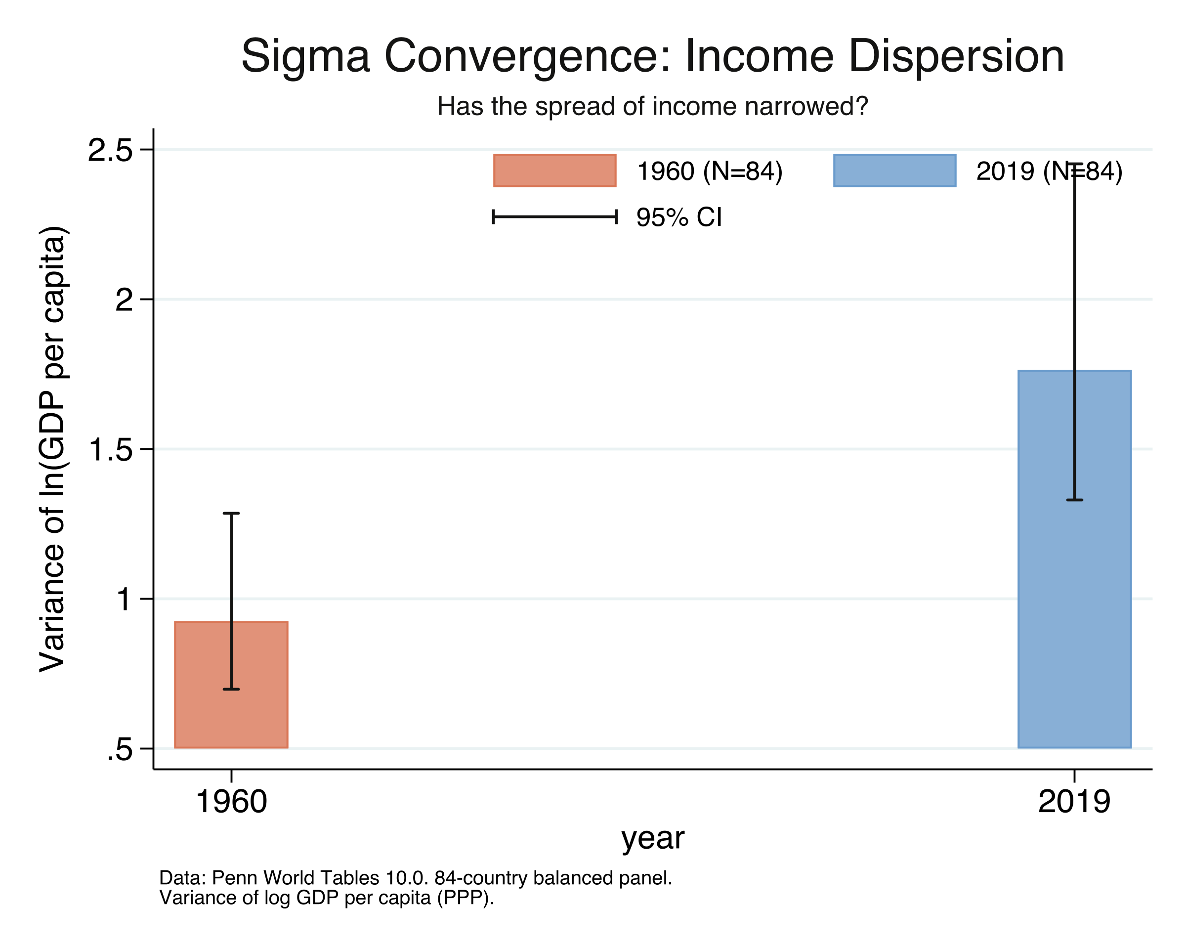
Variance of log GDP per capita, 1960 versus 2019 (same 84 countries), with chi-squared 95% CIs.

Here is the paradox made concrete. The variance of log income rose from 0.924 in 1960 to 1.764 in 2019 — up 90.8%, sigma divergence. A one-SD move in 2019 is a 3.8-fold difference in living standards, up from 2.6-fold in 1960. The error bars are asymmetric because the variance CI uses the chi-squared distribution. Poorer countries grow faster, yet the world spread widened.

Sigma followed beta with an 8-year lag — and only after 2008

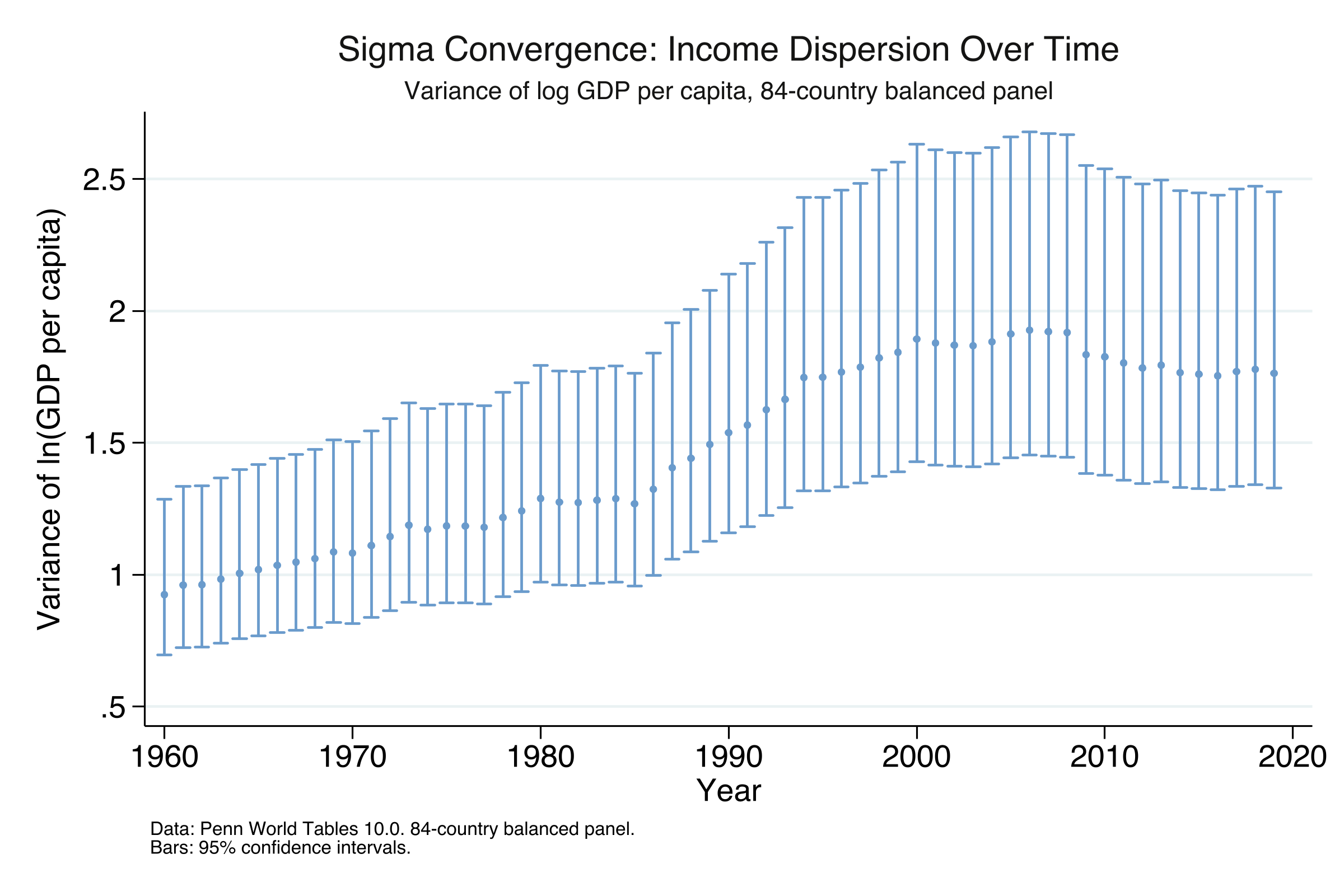
Year-by-year variance of log income (84-country panel). It peaks in 2008, then declines.

Beta turned to convergence around 2000, but the variance kept rising to a 1.918 peak in 2008 before falling 8.1% to 1.764 by 2019. That ~8-year gap is the Young–Higgins–Levy result in action: random shocks — crises, commodity swings, conflict — dispersed incomes faster than the catch-up tendency could pull them together, until the convergence force finally dominated.

Can poor countries grow faster and the gap widen? Yes — that’s the whole point

Objection. Surely faster growth at the bottom must shrink the spread — this looks like a contradiction.

Response. No. Beta convergence is the average tendency; sigma is the realized spread. Random shocks can widen the distribution even while the rear runners accelerate. Beta is necessary but not sufficient for sigma — exactly what 1960–2008 shows.

Steelman it first — the intuition that catch-up must narrow the spread is natural. The resolution is Young, Higgins & Levy (2008): the systematic catch-up force competes with the dispersing force of idiosyncratic shocks. Only when the former dominates does sigma fall — which is why sigma convergence didn’t begin until 2008, eight years after beta.

Robust across every window: red divergence before 2000, blue convergence after

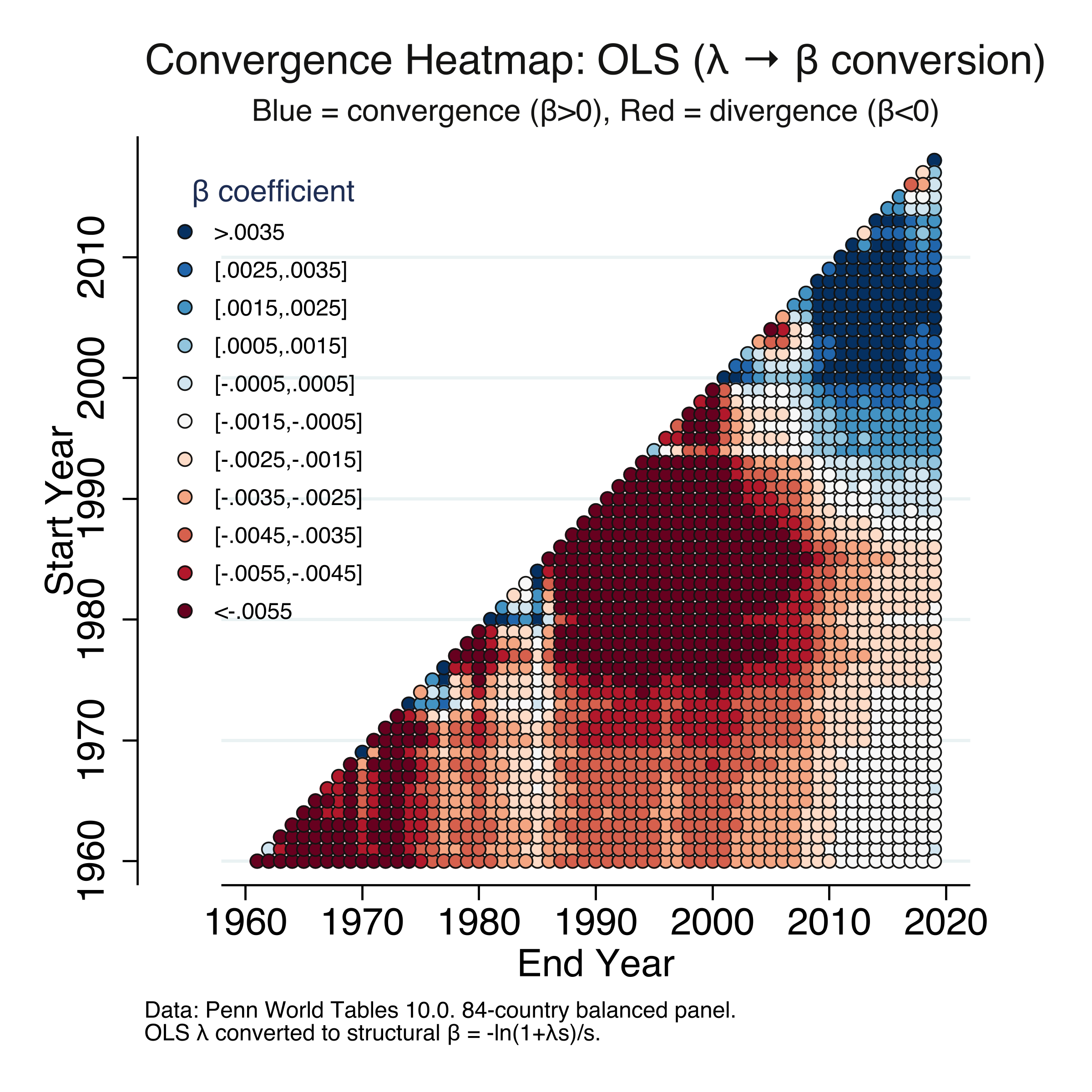
Convergence heatmap over all start/end-year pairs (OLS β; the NLS heatmap is virtually identical). Blue = convergence, red = divergence.

~1,770 regressions, one per window. The upper-right triangle (periods ending 2010–2019) is blue; central and lower-left regions (ending before 2000) are red. The crossover migrates gradually along diagonals. This is the ultimate robustness check: the convergence finding isn’t an artifact of cherry-picked endpoints. Short windows on the diagonal are noisier, as expected.

This is an association, not a causal effect — two assumptions still do the work

Objection. Does a negative slope prove that being poor causes faster growth?

Response. No. This is unconditional convergence — a descriptive association across countries, not an ATE. A causal reading needs controls for institutions, human capital, and policy; the regression deliberately omits them.

Be explicit about the estimand. We are describing a cross-country regularity, not identifying a treatment effect. Conditional convergence (the natural next step, and Exercise 2 in the post) adds those controls and asks whether the speed approaches the 2% benchmark. The honest claim here is correlational.

What it means: convergence is real, but far too slow to wait out

• Unconditional convergence is real since ~2000 — but at 0.36%/yr, a 190-year half-life
• Five times slower than the 2% conditional benchmark
• The 2019 income spread is still 91% wider than 1960’s
• Catch-up forces alone won’t close global gaps in any planning horizon

The policy reading: don’t count on automatic catch-up. At this pace the gaps persist for centuries. Active investment in education, infrastructure, institutions, and technology transfer remains essential — convergence is a tailwind, not an autopilot.

Let theory, not patience, close the gap — convergence is real, but glacially slow.

The single sentence to leave them with. Beta convergence after 2000 is genuine and statistically significant, but a 190-year half-life and a still-widening distribution mean it cannot substitute for active development policy. The optimistic hypothesis is finally true — and almost irrelevant on a human timescale without intervention.