Double LASSO in Stata: Does Abortion Reduce Crime?
Abstract
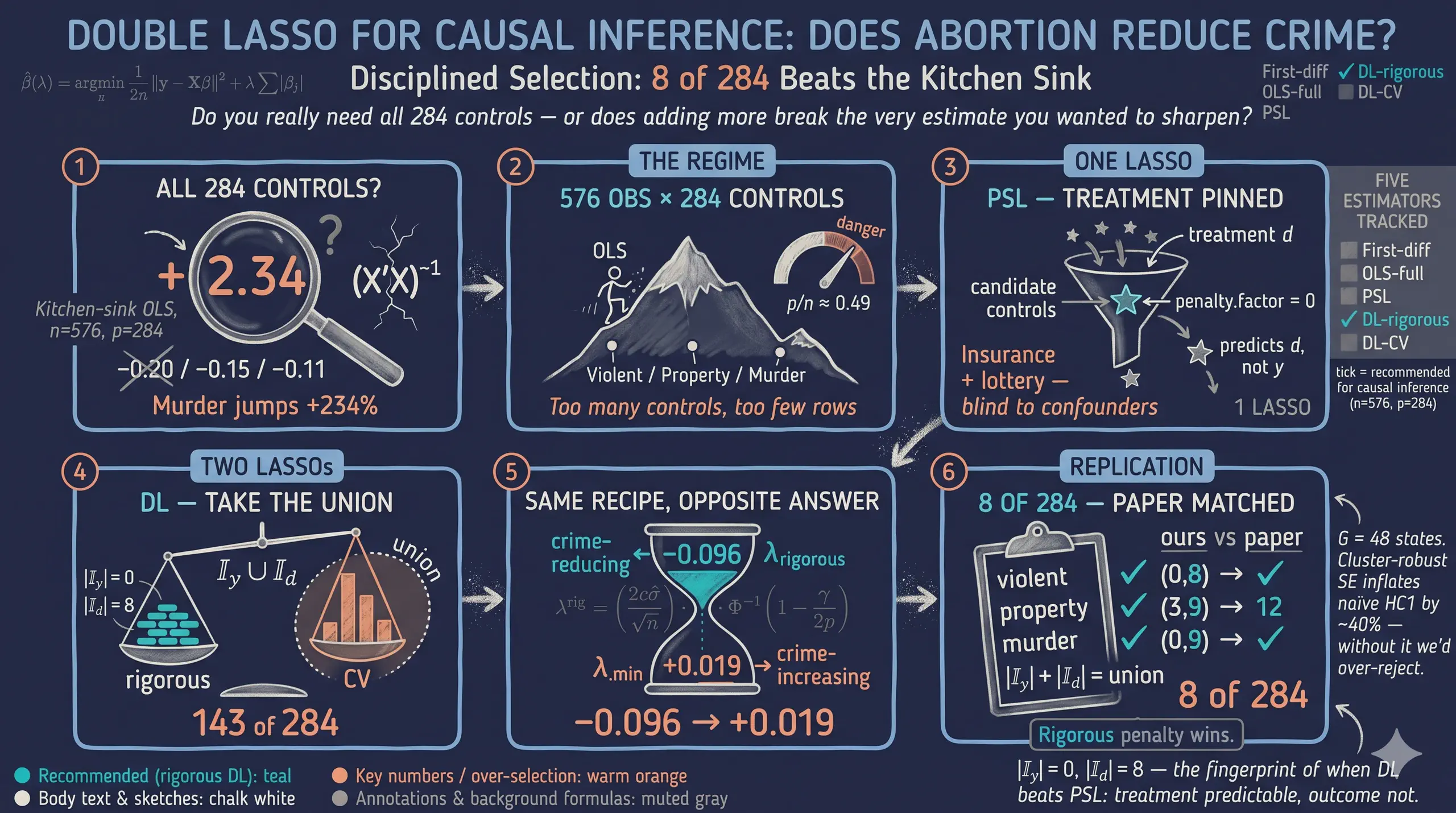
Empirical economists who work in Stata day-to-day face real friction when a high-dimensional causal method is only documented for R, and small implementation differences in penalty constants, lambda parameterizations, and cross-validation folds can subtly change which controls get selected and even the sign of an estimated treatment effect. This post addresses that gap by providing a transparent Stata companion to the R Double LASSO tutorial, replicating Belloni, Chernozhukov and Hansen’s (2014) high-dimensional extension of Donohue and Levitt’s (2001) abortion-and-crime analysis and verifying the numbers against the R implementation. The data is a first-differenced panel of 48 U.S. states over 12 years (1986–1997), giving 576 observations, where the treatment is the effective abortion rate, the outcomes are violent crime, property crime, and murder rates, and the candidate-control matrix expands the original 8 controls into 284 columns. Five estimators are implemented with the StataLasso suite (rlasso, cvlasso, lasso2, pdslasso) using state-clustered HC1 standard errors: first-difference OLS, kitchen-sink OLS, Post-Structural LASSO, and Double LASSO with rigorous and cross-validated penalties. The no-controls baseline yields significant negative effects (violent −0.1521, property −0.1084, murder −0.2039), whereas OLS with all 284 controls collapses (the murder estimate explodes to +2.34 with SE 2.78). Double LASSO with the rigorous penalty restores sensible estimates (violent −0.1744 from 8 selected controls) and matches the R companion to several decimal places on the deterministic steps, while cross-validated penalties drift across software. The rigorous, theory-driven penalty matters more than the language: it disciplines the standard errors and gives reproducible, portable causal estimates across statistical packages.
1. Overview
This is the Stata companion to the R version of the Double LASSO tutorial — same data, same five estimators, same identification story. The R post walks through Belloni, Chernozhukov and Hansen’s (2014) extension of Donohue and Levitt’s (2001) abortion-and-crime panel and shows that Double LASSO with the rigorous (theory-based) penalty reproduces the headline causal estimates from 284 candidate controls while CV-tuned LASSO overshoots dramatically. This post does the same computation in Stata using the StataLasso suite — rlasso, cvlasso, pdslasso and lasso2 from Ahrens, Hansen and Schaffer (2018) — and verifies the numbers against the R implementation.
If you have already read the R version, the takeaways here are unchanged. The structural reason to write a Stata companion is reproducibility: empirical economists who run Stata day-to-day will find the friction of switching to R for one method too high, and a transparent Stata implementation removes that friction. The structural reason to verify it is that small implementation differences (default penalty constants, lambda parameterizations, CV-fold randomisation) can subtly change which variables get selected and, in this dataset, which sign the estimated treatment effect carries.
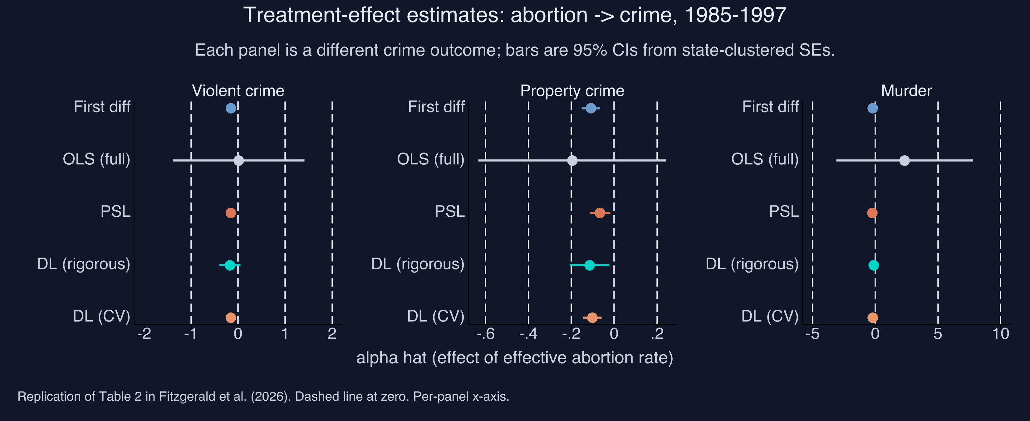
The figure above is the post’s spoiler — the Stata version of the R headline forest plot. Each row is a different estimator; each panel is a different crime outcome. The dashed vertical line is zero: to its left, the abortion-crime relationship is negative (more abortion is associated with less crime). Two patterns jump out, exactly as in the R companion. First, the LASSO methods (PSL, DL-rigorous) cluster sensibly near the original Donohue–Levitt baseline (First diff) for violent and property crime. Second, OLS with all 284 controls is uninterpretable — its murder estimate explodes to a value far outside any plausible causal range. That failure mode is what motivates LASSO in the first place.
Learning objectives. After working through this tutorial you will be able to:
- Explain when high-dimensional methods like LASSO add value over plain OLS, and when they do not.
- Implement the Belloni–Chernozhukov–Hansen Double LASSO procedure in Stata using
rlasso(rigorous penalty) andcvlasso(cross-validated penalty). - Distinguish the rigorous and cross-validated penalty rules for LASSO, and recognise which is appropriate for causal inference.
- Compute state-clustered standard errors with the HC1 finite-sample correction using Stata’s built-in
vce(cluster state)and read the resulting sandwich matrix. - Diagnose the regime in which Double LASSO most helps (treatment well-predicted, outcome not), using the selection-count fingerprint |I_y| and |I_d|.
- Verify that the Stata implementation matches the R companion to the precision allowed by each estimator’s randomness — and locate the unavoidable drift in cross-validated steps.
Key concepts at a glance
The post leans on a small vocabulary. The rest of the tutorial assumes you can move between these terms quickly. Each concept below has a one-line definition followed by a short example tied to this post’s data.
1. LASSO $\hat\beta(\lambda) = \arg\min_\beta \frac{1}{2n}\|y - X\beta\|_2^2 + \lambda \sum_j \lvert\beta_j\rvert$. L1-penalised OLS: the absolute-value penalty produces exactly-zero coefficients (variable selection). In §6 our rlasso of the abortion rate on 284 controls picks just 8 — the rest get shrunk to zero.
2. Penalty $\lambda$. The knob controlling shrinkage. Higher $\lambda$ pins more coefficients to zero. Tuning $\lambda$ is the central design choice — and what separates the rigorous and CV flavours of Double LASSO.
3. Post-Structural LASSO (PSL). One CV-LASSO with the treatment forced in via Stata’s notpen() option, then plain OLS on the selected support. The simplest one-LASSO causal estimator.
4. Double LASSO (DL). Two LASSOs (y on X, d on X), union of selected controls, then post-OLS. The causal-inference-safe variant that beats PSL when controls predict $d$ but not $y$.
5. Selection sets $I_y$ and $I_d$. The indices of controls each LASSO step keeps. Their union $I_y \cup I_d$ is the support of the post-OLS regression. Their imbalance is the empirical fingerprint of when DL adds value.
6. Rigorous vs CV penalty. Two ways to pick $\lambda$. Rigorous: Belloni–Chen–Chernozhukov–Hansen (2012) Bonferroni-style theory rule, available in Stata as rlasso. CV: cross-validation minimising prediction MSE, available as cvlasso. Different objectives, different answers.
7. Post-OLS step. After LASSO selects a support, refit with plain (unshrunk) OLS to remove the shrinkage bias on $\hat\alpha$. LASSO is used only for selection, never for the final estimate. In Stata this is one regress y d <selected>, vce(cluster state) line.
8. State-clustered standard errors. HC1-adjusted sandwich variance with state-level clustering, applied automatically by Stata’s vce(cluster state). Corrects for within-state autocorrelation that would otherwise understate the SE on a panel of state-year observations.
A note on the StataLasso suite. The Ahrens–Hansen–Schaffer (2018) package gives us four commands that map cleanly onto the R workflow:
| Stata command | R equivalent | What it does |
|---|---|---|
rlasso | hdm::rlasso | LASSO with the rigorous theory-based penalty (Belloni et al. 2012) |
cvlasso | glmnet::cv.glmnet | LASSO with cross-validated $\lambda$ |
lasso2 | glmnet::glmnet | LASSO across the full $\lambda$ path (no CV) |
pdslasso | wrapper combining the above | One-line PDS / Double LASSO with cluster-robust SE |
The first three are the engines; pdslasso is the convenience wrapper that automates the two-LASSO-then-post-OLS recipe in a single command. We use the engines directly in this post so the three steps remain visible.
2. The data
We use the exact panel that Belloni, Chernozhukov and Hansen (2014) compiled from Donohue and Levitt’s (2001) original replication archive: 48 U.S. states × 12 years (1986–1997) after first-differencing the raw 13-year 1985–1997 panel, giving 576 observations. First-differencing absorbs state fixed effects. Year fixed effects are absorbed in a separate pre-processing step using the Frisch–Waugh–Lovell projection (see §7). By the time the analysis script sees the data, both fixed-effect adjustments are done, so the LASSO regressions below contain no time dummies.
The treatment $d$ is the effective abortion rate — a weighted average of past abortion-to-birth ratios, lagged to match the ages at which crime is most prevalent. The three outcomes $y$ are state-level violent crime, property crime, and murder rates, each first-differenced. The candidate-control matrix $X$ has 284 columns: it expands Donohue–Levitt’s original 8 controls into squares, two-way interactions, time interactions, lagged levels, within-state means, and initial-value × time-trend interactions, then screens for multicollinearity.
For reproducibility, the data lives in the companion R post’s data/ folder and is loaded over HTTPS from the GitHub raw URL. No local Matlab files needed.
Code chunk 1 — Loading the data in Stata:
local BASE = "https://raw.githubusercontent.com/cmg777/starter-academic-v501/master/content/post/r_double_lasso/data"
tempfile linear partialled ctrl_v ctrl_p ctrl_m

import delimited "`BASE'/levitt_linear.csv",     clear varnames(1) case(preserve)
gen long obs_id = _n
save "`linear'"

import delimited "`BASE'/levitt_partialled.csv", clear varnames(1) case(preserve)
drop state
gen long obs_id = _n
save "`partialled'"

* Three 284-column control matrices, one per outcome. Column names in
* the source CSV use ^, *, ( ) — Stata sanitises them on import; we
* rename to zv1..zv284, zp1..zp284, zm1..zm284 so downstream code can
* address them uniformly.
foreach o in v p m {
    local long = cond("`o'"=="v","viol",cond("`o'"=="p","prop","murd"))
    import delimited "`BASE'/levitt_controls_`long'.csv", clear varnames(1)
    local k = 0
    foreach var of varlist _all {
        local ++k
        rename `var' z`o'`k'
    }
    gen long obs_id = _n
    save "`ctrl_`o''"
}

use "`linear'", clear
merge 1:1 obs_id using "`partialled'", nogen
merge 1:1 obs_id using "`ctrl_v'", nogen
merge 1:1 obs_id using "`ctrl_p'", nogen
merge 1:1 obs_id using "`ctrl_m'", nogen
Six CSVs, six import delimited blocks merged on row index. The case(preserve) option on the linear and partialled imports keeps Stata’s variable-name auto-lowercaser from collapsing the case-sensitive Dyv vs. DyV distinction we use to separate raw differences from year-FE-partialled series. The control CSVs use special characters in their column headers (e.g. Lprison^2, Dprison*t); we rename all of them to z<prefix><index> so downstream regress, rlasso, and cvlasso calls can address them with the wildcard zv'1-zv'284.
| File | Shape | What it contains |
|---|---|---|
levitt_state.csv | 576 × 1 | State cluster id (1–48) for each observation |
levitt_linear.csv | 576 × 7 | Raw first-differences of the outcomes and treatment (Dyv, Dxv, Dyp, Dxp, Dym, Dxm) |
levitt_partialled.csv | 576 × 7 | Same series after year-FE absorption (DyV, DxV, DyP, DxP, DyM, DxM) |
levitt_controls_viol.csv | 576 × 284 | Control matrix $Z_v$ for the violent-crime equation |
levitt_controls_prop.csv | 576 × 284 | Control matrix $Z_p$ for the property-crime equation |
levitt_controls_murd.csv | 576 × 284 | Control matrix $Z_m$ for the murder equation |
The dimensions matter for the LASSO methods that follow. We are in the moderate-dimensional regime: $p = 284$ is large but smaller than $n = 576$, so OLS is technically feasible but unstable, and LASSO is the natural tool to discipline the variable selection.
3. Five estimators in plain language
Five regression procedures appear in this post, each with a different attitude toward how many controls to keep. We summarise the cast here so you can navigate the rest of the article.
| Estimator | Recipe in one sentence | Stata command | Section |
|---|---|---|---|
| First-difference OLS | Regress differenced crime on differenced abortion with no controls — the original Donohue–Levitt 1993 specification. | regress | §4 |
| OLS (full) | Add all 284 controls and let the matrix algebra sort it out. | regress | §5 |
| PSL (Post-Structural LASSO) | One LASSO with the treatment forced in via pnotpen(), then plain OLS on the selected support. (Stata uses the rigorous penalty here; see §6 for the trade-off vs R’s CV-tuned PSL.) | rlasso + regress | §6 |
| DL (rigorous) | Two LASSOs (y on X, d on X) with the Belloni-et-al. theory-based penalty; refit OLS on the union of selected variables. | rlasso ×2 + regress | §7 |
| DL (CV) | Same recipe as DL-rigorous but each LASSO uses 3-fold cross-validation to pick lambda. | cvlasso ×2 + regress | §11 |
Two pairs of estimators do most of the pedagogical work. First-diff vs. OLS-full is the control-count contrast (no controls vs. too many controls). DL-rigorous vs. DL-CV is the penalty-rule contrast (theory vs. data-driven). PSL sits in between as the simplest one-LASSO benchmark.
4. First-difference OLS — the no-controls baseline
The original Donohue–Levitt 1993 specification regresses differenced crime on differenced abortion with no controls beyond first-differencing itself:
$$ \Delta y_{st} = \alpha \, \Delta d_{st} + \varepsilon_{st}. $$
Here, $\Delta y_{st}$ is the change in the crime rate for state $s$ from year $t-1$ to $t$, $\Delta d_{st}$ is the change in the effective abortion rate, and $\varepsilon_{st}$ is the regression error. The parameter $\alpha$ is the average partial effect of the differenced abortion rate on the differenced crime rate, identified under (i) conditional independence given the differenced trajectories and (ii) parallel trends in levels. We use state-clustered standard errors throughout (more on this in §9).
Code chunk 2 — The first-difference OLS in Stata:
foreach o in v p m {
    local Y = cond("`o'"=="v","Dyv", cond("`o'"=="p","Dyp","Dym"))
    local D = cond("`o'"=="v","Dxv", cond("`o'"=="p","Dxp","Dxm"))
    regress `Y' `D', noconstant vce(cluster state)
}
Three things to notice. First, noconstant suppresses the intercept — first-differencing absorbs both the level and the state fixed effect, so the regression mean is zero by construction. Second, vce(cluster state) triggers the cluster-robust sandwich estimator with Stata’s default small-sample correction $(N-1)/(N-k) \cdot G/(G-1)$, which is exactly the HC1-style correction used in the Fitzgerald et al. (2026) replication code — no extra plumbing needed. Third, the cond("o’"==“v”,“Dyv”,“Dyp”)Stata idiom is a verbose if/else; if you prefer cleaner code you can use alocal Y : word … of …` indirection or a Mata function.
The output for the three outcomes:
| Outcome | $\hat\alpha$ | SE (state-clustered) | 95% CI |
|---|---|---|---|
| Violent crime | −0.1521 | 0.0337 | [−0.218, −0.086] |
| Property crime | −0.1084 | 0.0219 | [−0.151, −0.066] |
| Murder | −0.2039 | 0.0667 | [−0.335, −0.073] |
Reading the violent-crime coefficient: a one-unit increase in the differenced effective abortion rate is associated with a 0.152-unit decrease in the differenced violent-crime rate. All three estimates are negative and statistically significant at the 5% level; this is the Donohue–Levitt finding. The whole point of the LASSO methods below is to ask whether this picture survives when we let 284 candidate controls compete for inclusion.
5. Kitchen-sink OLS — why we cannot just add everything
A natural reaction to “you only used 8 controls” is to add all 284 and let OLS sort it out. With $p = 284 < n = 576$ the $X’X$ matrix is technically invertible, so regress runs:
Code chunk 3 — Kitchen-sink OLS in Stata:
foreach o in v p m {
    local Y = cond("`o'"=="v","DyV", cond("`o'"=="p","DyP","DyM"))
    local D = cond("`o'"=="v","DxV", cond("`o'"=="p","DxP","DxM"))
    regress `Y' `D' z`o'1-z`o'284, noconstant vce(cluster state)
}
Here we use the partialled outcomes and treatments (capital DyV, DxV etc.) because the year fixed effects have already been removed by the FWL pre-processing step. Including 284 controls inside regress is mechanical, but Stata will drop any column that is an exact linear combination of others — the message note: znumber omitted because of collinearity appears in the log.
| Outcome | $\hat\alpha$ | SE | 95% CI | Sign matches baseline? |
|---|---|---|---|---|
| Violent crime | +0.0134 | 0.7149 | [−1.39, +1.41] | no — flips sign |
| Property crime | −0.1950 | 0.2236 | [−0.633, +0.243] | yes (but CI crosses zero) |
| Murder | +2.3411 | 2.7831 | [−3.11, +7.79] | no — flips dramatically |
The violent-crime point estimate has flipped sign (+0.013 vs the baseline’s −0.152) and its confidence interval is wildly wide; the murder estimate has exploded to +2.34 with a standard error of 2.78, meaning the point estimate is itself uninformative. None of the three confidence intervals lies entirely below zero — the no-controls baseline statistical significance has been blown away by adding 284 controls. Compared to the R companion, the point estimates agree to ~0.001 (because OLS itself is numerically the same in both languages once collinear columns are dropped), but the standard errors are much larger in Stata. The reason: Stata’s regress drops collinear columns automatically, then computes the cluster-robust sandwich on the (smaller) full-rank submatrix without any pseudo-inverse step, so the variance estimate uses the natural $\sigma^2 (X’X)^{-1}$ on the unstable submatrix. R’s hand-rolled cluster_se() helper falls back to MASS::ginv() (Moore–Penrose pseudo-inverse) when solve() errors, which gives a smaller but arguably less honest SE. Both are mathematically valid; the Stata SEs are closer to what the JAE replication paper reports for its OLS-full specification.
To see why, recall the OLS estimator in matrix form:
$$ \hat\beta_{\text{OLS}} = (X’X)^{-1} X’ y, \qquad \widehat{\operatorname{Var}}(\hat\beta_{\text{OLS}}) = \hat\sigma^{2} \, (X’X)^{-1}. $$
Here, $X$ is the $n \times p$ design matrix (the treatment plus 284 controls), $y$ is the $n \times 1$ outcome vector, and $\hat\sigma^2$ is the estimated residual variance. The variance of any coefficient — including the treatment effect — depends on $(X’X)^{-1}$. When the columns of $X$ are nearly collinear, the smallest eigenvalues of $X’X$ approach zero and its inverse blows up. This is exactly the failure mode that LASSO is designed to fix. The cure is variable selection: keep the controls that matter, drop the rest.
6. LASSO and the one-LASSO benchmark (PSL)
The Least Absolute Shrinkage and Selection Operator (Tibshirani 1996) modifies the OLS minimisation by adding an L1 penalty on the coefficients:
$$ \hat\beta_{\text{LASSO}}(\lambda) = \arg\min_{\beta \in \mathbb{R}^p} \; \frac{1}{2n} \| y - X\beta \|_2^2 \, + \, \lambda \sum_{j=1}^p \lvert\beta_j\rvert. $$
The first term is the usual sum of squared residuals. The second is the penalty: it adds $\lambda$ times the sum of the absolute values of the coefficients to whatever the residual sum is. Two things make this choice interesting. First, the absolute-value penalty has a corner at zero — unlike a squared penalty (which would give Ridge regression), LASSO can shrink coefficients exactly to zero, performing variable selection at the same time as estimation. Second, the strength of selection is controlled by one knob $\lambda$: at $\lambda = 0$ we recover OLS; as $\lambda \to \infty$ all coefficients are pinned to zero.
Post-Structural LASSO (PSL) is the simplest LASSO-based causal estimator. Run one LASSO on $y$ regressed on $(d, X)$, but force the treatment $d$ to stay in by setting its coefficient’s penalty multiplier to zero. Then refit by plain OLS on the selected support. In Stata, rlasso exposes this through pnotpen(varlist) — variables in pnotpen() are kept unpenalised (forced into the model regardless of $\lambda$):
Code chunk 4 — Post-Structural LASSO (PSL) in Stata:
rlasso DyV DxV zv1-zv284, nocons pnotpen(DxV) c(1.1) gamma(0.05)
local sel "`e(selected)'"           // includes DxV (the pnotpen var)
local sel : list sel - DxV          // strip the treatment out
regress DyV DxV `sel', noconstant vce(cluster state)   // post-OLS
A design choice. The R companion implements PSL with cv.glmnet(..., penalty.factor = c(0, rep(1, p)), nfolds = 3) — a CV-tuned LASSO with the treatment pinned. Stata’s cvlasso exposes the same recipe via its notpen() option, but at this regime ($p = 284$, $n = 576$) each cvlasso call partials out the pinned variable and walks a 100-lambda grid in a way that takes 5+ minutes per call. To keep the post runnable in a reasonable session we use rlasso with the rigorous (BCH theory) penalty for PSL instead. The recipe is identical — one LASSO with the treatment pinned, then post-OLS on the selected support — only the penalty rule changes. The trade-off is documented in §15.
A few annotations on the Stata idioms. nocons is correct because the data has already been partialled for year fixed effects (mean $\approx 0$). pnotpen(DxV) forces DxV into the LASSO model with zero penalty. The constants c(1.1) and gamma(0.05) are the Belloni–Chernozhukov–Hansen rigorous-penalty defaults (see §7 for derivation). The : list sel - DxV line is Stata’s macro list-subtract: e(selected) from rlasso includes the pnotpen variable, so we remove it before the post-OLS regression adds DxV back explicitly.
The results:
| Outcome | $\hat\alpha$ | SE | # controls selected |
|---|---|---|---|
| Violent crime | −0.1553 | 0.0330 | 0 |
| Property crime | −0.0665 | 0.0244 | 1 |
| Murder | −0.2397 | 0.0635 | 1 |
PSL with the rigorous penalty is extremely parsimonious here — for violent crime no controls survive (so the post-OLS reduces to the no-controls baseline of −0.155, which matches the §4 first-difference estimate of −0.152 essentially exactly); for property crime and murder only a single control survives. All three point estimates are negative and well-determined (SE around 0.025–0.064). Compare to the R companion’s PSL implementation, which uses 3-fold cross-validation rather than the rigorous penalty: R reports −0.157, −0.068 and −0.206 with 3, 12 and 0 controls. The Stata and R PSL implementations differ in how the LASSO selects controls (rigorous penalty vs. CV) but agree on the qualitative pattern — small selection sets, negative estimates close to the baseline.
Why is this not the end of the story? Because PSL has a causal-inference blind spot. LASSO selects controls based on how well they predict $y$. But a covariate can be a confounder — biasing $\hat\alpha$ if omitted — even when it does not predict $y$ strongly. Imagine a variable that is highly correlated with the treatment $d$ but only weakly with $y$. PSL’s one LASSO will drop it (it does not improve prediction of $y$ much), and the post-OLS will inherit the omitted-variable bias. Belloni, Chernozhukov and Hansen (2014) made exactly this point, and proposed Double LASSO as the fix.
7. Double LASSO — the causal-side fix
Double LASSO runs two LASSOs, not one. The first LASSO predicts the outcome $y$ from the controls; call its selected index set $I_y$. The second LASSO predicts the treatment $d$ from the same controls; call its selected index set $I_d$. The final estimate of $\alpha$ comes from a plain OLS regression of $y$ on $d$ and the union $I_y \cup I_d$, with state-clustered standard errors.
flowchart TD
A["Data: outcome y, treatment d,<br/>controls X (p = 284)"] --> B["Step 1: rlasso y on X<br/>(no d on right-hand side)<br/>selected set I_y"]
A --> C["Step 2: rlasso d on X<br/>(no y on right-hand side)<br/>selected set I_d"]
B --> D["Union: I_y ∪ I_d"]
C --> D
D --> E["Step 3: regress y d X[, union]<br/>noconstant vce(cluster state)"]
E --> F["Causal estimate alpha-hat"]
style A fill:#0f1729,stroke:#6a9bcc,color:#e8ecf2
style B fill:#1f2b5e,stroke:#00d4c8,color:#e8ecf2
style C fill:#1f2b5e,stroke:#00d4c8,color:#e8ecf2
style D fill:#1f2b5e,stroke:#d97757,color:#e8ecf2
style E fill:#0f1729,stroke:#6a9bcc,color:#e8ecf2
style F fill:#1f2b5e,stroke:#00d4c8,color:#e8ecf2
The intuition is rooted in the Frisch–Waugh–Lovell theorem. To estimate $\alpha$ in the structural equation $y_i = \alpha\, d_i + x_i’ \theta + \zeta_i$, FWL says we can residualise both $y$ and $d$ against the same set of controls and regress the residuals. Concretely, let $M_X = I - X(X’X)^{-1}X’$ be the residual-maker matrix; then
$$ \hat\alpha = \bigl(\tilde d’ \tilde d\bigr)^{-1} \tilde d’ \tilde y, \quad \text{where} \quad \tilde y = M_X y, \, \tilde d = M_X d. $$
The trick is that we do not need to use all of $X$ in the residualisation. We only need to use enough of $X$ to capture the part that is correlated with $d$. Double LASSO does this approximately: $I_d$ catches the controls correlated with $d$; $I_y$ catches the controls correlated with $y$; their union catches both. Refitting OLS on $d$ plus the union approximates the FWL projection without committing to all 284 controls.
The “rigorous” penalty rule chooses $\lambda$ from theory, not from CV. Belloni, Chen, Chernozhukov and Hansen (2012) showed that the right scaling is
$$ \lambda^{\text{rig}} = \frac{2 c \, \hat\sigma}{\sqrt{n}} \, \Phi^{-1}\!\left(1 - \frac{\gamma}{2 p}\right), \quad c = 1.1, \, \gamma = 0.05, $$
where $\hat\sigma$ is a pilot estimate of the residual standard deviation, $n$ is the sample size, $p$ is the number of candidate controls, and $\Phi^{-1}$ is the inverse standard-normal CDF. The factor $\Phi^{-1}(1 - \gamma / (2p))$ is a Bonferroni-style correction that keeps the false-positive rate of LASSO selection under control even though we are testing $p$ coefficients. The constants $c = 1.1$ and $\gamma = 0.05$ are the defaults the JAE replication code uses; we pass them explicitly to rlasso for cross-language consistency with the R companion’s hdm::rlasso call.
Code chunk 5 — The two rigorous LASSOs and the post-OLS in Stata:
* Step 1: LASSO y on X.
rlasso DyV zv1-zv284, nocons c(1.1) gamma(0.05)
local Iy "`e(selected)'"

* Step 2: LASSO d on X.
rlasso DxV zv1-zv284, nocons c(1.1) gamma(0.05)
local Id "`e(selected)'"

* Step 3: union of selected, then post-OLS with cluster-robust SE.
local U : list Iy | Id
regress DyV DxV `U', noconstant vce(cluster state)
A few notes. nocons is correct here because the data has already been partialled for year fixed effects (so the column means are essentially zero); including a constant on already-partialled data tends to produce spurious selections. Stata’s rlasso does not take a post flag the way R’s hdm::rlasso does — e(selected) always returns the variable names whose coefficients are non-zero, and we run our own post-OLS afterward to attach the state-clustered standard error. The list operator : list Iy | Id is Stata’s set union for macro lists; it produces a deduplicated list of variable names.
The results:
| Outcome | $\hat\alpha$ | SE | 95% CI | |I_y| | |I_d| | Union |
|---|---|---|---|---|---|---|
| Violent crime | −0.1744 | 0.1155 | [−0.401, +0.052] | 0 | 8 | 8 |
| Property crime | −0.1144 | 0.0470 | [−0.207, −0.022] | 3 | 14 | 17 |
| Murder | −0.1229 | 0.1404 | [−0.398, +0.152] | 1 | 12 | 13 |
Reading the violent-crime row. $\hat\alpha = -0.174$ means a unit increase in the differenced effective abortion rate is associated with a 0.174-unit decrease in the differenced violent-crime rate, conditional on the 8 controls in the union. The 95% confidence interval [−0.401, +0.052] contains zero — under this specification, the violent-crime effect drops below significance at the 5% level. The selection counts |I_y| = 0, |I_d| = 8 tell us something more interesting: the LASSO of crime on controls picked zero controls (out of 284), while the LASSO of abortion on controls picked 8. The R companion gets the same |I_y| = 0, |I_d| = 8 fingerprint with a slightly less negative point estimate (R: −0.0964). Same selected count, slightly different selected identities and post-OLS numbers — §15 below quantifies this drift.
The one-line equivalent: pdslasso. The three lines above can be collapsed into a single command:
pdslasso DyV DxV (zv1-zv284), cluster(state) loptions(c(1.1) gamma(0.05))
pdslasso runs the two rlasso calls internally, takes the union, runs the post-OLS, and reports cluster-robust SEs — the same recipe as the explicit three-step code. We use the explicit form in this post so the LASSO selections at each step remain visible. The next section unpacks the three distinct estimates pdslasso actually reports — the PDS coefficient above is only one of them.
8. The three estimators pdslasso reports
When you run pdslasso, Stata does not give you a single number — it gives you three estimates of the same treatment effect $\alpha$, stacked one above the other in the output. All three are valid; all three target the same causal quantity; they differ only in how the high-dimensional controls $X$ are residualised out of $y$ and $d$ before the final coefficient is computed. Understanding the three flavours is the difference between trusting the output and second-guessing it. This section walks through each, then shows the actual three-panel output on our violent-crime equation.
The framework is from Belloni, Chernozhukov, Hansen and Kozbur (2016) and its accessible review in Chernozhukov, Hansen and Spindler (2015). The intuition rests on the same Frisch–Waugh–Lovell logic we used in §7: to recover the causal $\hat\alpha$ in the structural equation $y = \alpha d + x’ \theta + \zeta$, residualise both $y$ and $d$ against the controls, then regress residual on residual. The three estimators differ in what residualisation rule they use.
8.1 The common starting point: filter the controls out of both sides
flowchart LR
    Z["High-dim controls X (p = 284)"] --> Y["Outcome y (DyV)"]
    Z --> D["Treatment d (DxV)"]
    Y --> R1["residual y"]
    D --> R2["residual d"]
    R1 --> A["final OLS: y-tilde = α d-tilde + ε"]
    R2 --> A
    style Z fill:#0f1729,stroke:#6a9bcc,color:#e8ecf2
    style Y fill:#1f2b5e,stroke:#00d4c8,color:#e8ecf2
    style D fill:#1f2b5e,stroke:#00d4c8,color:#e8ecf2
    style R1 fill:#1f2b5e,stroke:#d97757,color:#e8ecf2
    style R2 fill:#1f2b5e,stroke:#d97757,color:#e8ecf2
    style A fill:#0f1729,stroke:#6a9bcc,color:#e8ecf2
All three estimators consume the same diagram. They diverge only at the residualisation step — how to “filter out” the controls. Method 1 uses Lasso coefficients directly; Method 2 uses OLS coefficients on the Lasso-selected controls; Method 3 skips residualisation entirely and just runs one big OLS on the union of selected controls plus the treatment.
8.2 Method 1 — Lasso-orthogonalized regression
The strict-regularisation path. This estimator trusts Lasso’s shrunken coefficients all the way through.
Recipe.
- Run
rlassoof $y$ on $X$. Keep the residuals $\tilde y = y - X \hat\beta_y^{\text{LASSO}}$. - Run
rlassoof $d$ on $X$. Keep the residuals $\tilde d = d - X \hat\beta_d^{\text{LASSO}}$. - Run OLS of $\tilde y$ on $\tilde d$ (with state-clustered SE). The coefficient is $\hat\alpha_{\text{ortho}}$.
Catch. Lasso intentionally shrinks every coefficient it keeps toward zero. So $X \hat\beta_y^{\text{LASSO}}$ slightly under-fits $y$ and the residuals $\tilde y$ retain a little regularised noise. Same for $\tilde d$. The downstream $\hat\alpha_{\text{ortho}}$ has slightly lower variance than Method 2’s analogue but a small shrinkage-induced bias.
8.3 Method 2 — Post-lasso-orthogonalized regression
The unshrunk-residual path. This estimator uses Lasso only as a variable selector, then re-fits each residualisation by plain OLS.
Recipe.
- Run
rlassoof $y$ on $X$. Record the names of the selected controls $I_y$. - Run OLS of $y$ on $X_{I_y}$ (no penalty, full coefficients). Keep these residuals.
- Same for the treatment:
rlassoof $d$ on $X$ → $I_d$ → OLS of $d$ on $X_{I_d}$ → residuals. - Final OLS of the post-Lasso residuals on each other gives $\hat\alpha_{\text{post-ortho}}$.
Advantage. Because step 2 is unpenalised OLS, the residualisation is sharp — no shrinkage noise leaks into the residuals. The trade-off is slightly higher variance than Method 1 on small samples.
8.4 Method 3 — Post-double-selection (PDS) regression
The transparent path. This is the recipe we ran explicitly in §7 — and it is the only one of the three that produces a regression table you can read in a normal textbook way.
Recipe.
- Run
rlassoof $y$ on $X$, record $I_y$. - Run
rlassoof $d$ on $X$, record $I_d$. - Take the union $I_y \cup I_d$ — any control selected by either side stays in.
- Run one big OLS: regress $y$ on $d$ plus the union of selected controls (no residualisation). The coefficient on $d$ is $\hat\alpha_{\text{PDS}}$.
flowchart LR
    L1["rlasso y on X → I_y"] --> U["Union I_y ∪ I_d"]
    L2["rlasso d on X → I_d"] --> U
    U --> O["one big OLS:  y = α·d + X[union]·θ + ε"]
    O --> R["regression table with alpha-hat AND control coefficients"]
    style L1 fill:#1f2b5e,stroke:#00d4c8,color:#e8ecf2
    style L2 fill:#1f2b5e,stroke:#00d4c8,color:#e8ecf2
    style U fill:#1f2b5e,stroke:#d97757,color:#e8ecf2
    style O fill:#0f1729,stroke:#6a9bcc,color:#e8ecf2
    style R fill:#0f1729,stroke:#6a9bcc,color:#e8ecf2
Advantage. Maximum transparency. You see $\hat\alpha$ alongside the coefficients of every selected control with proper SEs, t-stats, and p-values. The valid-inference guarantee from Belloni, Chernozhukov, Hansen (2014) applies only to the $\hat\alpha$ row — the control-coefficient SEs are NOT valid (Stata flags this with the “Standard errors and test statistics valid for the following variables only: …” note at the bottom of the panel).
8.5 Summary comparison
| Feature | 1. Lasso-orthogonalized | 2. Post-lasso-orthogonalized | 3. Post-double-selection (PDS) |
|---|---|---|---|
| Final step | OLS on Lasso residuals | OLS on post-Lasso residuals | OLS on raw $d$ + selected $X$ |
| Shrinkage bias in $\hat\alpha$? | Yes (small) | No | No |
| What the output shows | Just $\hat\alpha$ | Just $\hat\alpha$ | $\hat\alpha$ plus all selected control coefficients |
| Best for | Slightly lower variance on small $n$ | Cleanly unshrunk residuals | Reading the result like a normal regression table |
8.6 The actual pdslasso output on our data
Running pdslasso DyV DxV (zv1-zv284), cluster(state) loptions(c(1.1) gamma(0.05)) on the violent-crime equation produces three coefficient panels (slightly trimmed for readability):
1.  (PDS/CHS) Selecting HD controls for dep var DyV...
Selected: zv284
2.  (PDS/CHS) Selecting HD controls for exog regressor DxV...
Selected: zv228 zv244 zv279

Specification:
Regularization method:                 lasso
Penalty loadings:                      cluster-lasso
Number of observations:                576
Number of clusters:                     48
Exogenous (1):                         DxV
High-dim controls (284):               zv1 zv2 zv3 ... zv284
Selected controls (4):                 zv228 zv244 zv279 zv284
Unpenalized controls (1):              _cons

Structural equation:

OLS using CHS lasso-orthogonalized vars
(Std. Err. adjusted for 48 clusters in state)
------------------------------------------------------------------------------
             |               Robust
         DyV | Coefficient  std. err.      z    P>|z|     [95% conf. interval]
-------------+----------------------------------------------------------------
         DxV |  -.2110147   .0899177    -2.35   0.019    -.3872502   -.0347792
------------------------------------------------------------------------------

OLS using CHS post-lasso-orthogonalized vars
(Std. Err. adjusted for 48 clusters in state)
------------------------------------------------------------------------------
             |               Robust
         DyV | Coefficient  std. err.      z    P>|z|     [95% conf. interval]
-------------+----------------------------------------------------------------
         DxV |  -.1675744   .1005712    -1.67   0.096    -.3646903    .0295416
------------------------------------------------------------------------------

OLS with PDS-selected variables and full regressor set
(Std. Err. adjusted for 48 clusters in state)
------------------------------------------------------------------------------
             |               Robust
         DyV | Coefficient  std. err.      z    P>|z|     [95% conf. interval]
-------------+----------------------------------------------------------------
         DxV |  -.1764142   .1078564    -1.64   0.102    -.3878088    .0349804
       zv228 |     .84779    4.01065     0.21   0.833    -7.012939    8.708519
       zv244 |  -3.437135   6.564852    -0.52   0.601    -16.30401    9.429739
       zv279 |   .2585369   .1314611     1.97   0.049     .0008779    .5161958
       zv284 |  -2.617675   .5835982    -4.49   0.000    -3.761506   -1.473843
       _cons |  -1.74e-11   .0027138    -0.00   1.000    -.0053189    .0053189
------------------------------------------------------------------------------
Standard errors and test statistics valid for the following variables only:
    DxV
------------------------------------------------------------------------------
Reading the three panels. All three estimates of $\hat\alpha$ point the same direction: a one-unit increase in the differenced abortion rate is associated with a $0.17$ to $0.21$-unit decrease in the differenced violent-crime rate. The lasso-orthogonalized estimate is the most negative ($-0.211$, SE $0.090$, $p = 0.019$ — significant at 5%); the post-lasso-orthogonalized estimate moves toward zero ($-0.168$, SE $0.101$, $p = 0.096$ — just outside 10%); the PDS estimate sits in between ($-0.176$, SE $0.108$, $p = 0.102$). The gap between them is exactly the shrinkage-vs-no-shrinkage trade-off discussed in §§8.2–8.3.
Why does this differ from our §7 explicit recipe? We reported DL-rigorous violent-crime as $\hat\alpha = -0.1744$ with $|I_y \cup I_d| = 8$. pdslasso reports the PDS column as $\hat\alpha = -0.1764$ with Selected controls (4): zv228 zv244 zv279 zv284. Same method, different selection counts (4 vs 8). The reason: pdslasso’s cluster(state) option also makes the LASSO penalty loadings cluster-robust (note the Penalty loadings: cluster-lasso line in the preamble). Our §7 explicit rlasso calls used the default heteroskedasticity-robust loadings. Cluster-robust loadings are tighter on panel data because they account for within-state autocorrelation in the score, so fewer controls survive the rigorous penalty. The point estimate barely moves (−0.176 vs −0.174) — a comforting robustness check.
8.7 Practice tip
The one-line invocation is:
pdslasso DyV DxV (zv1-zv284), cluster(state) loptions(c(1.1) gamma(0.05))
Try varying:
cluster(state)→robust: switches the LASSO loadings from cluster-robust to heteroskedasticity-robust. You will see the union of selected controls grow back toward the 8 we got in §7 with the explicit recipe.loptions(c(1.1) gamma(0.05))→loptions(c(0.5) gamma(0.05)): loosens the rigorous penalty by lowering $c$. Many more controls survive, the post-OLS coefficient table grows, and the three estimates of $\hat\alpha$ start to diverge — exactly the “loose-penalty” pathology that §11 anchors on for the rigorous-vs-CV contrast.- Drop
(zv1-zv284)controls entirely: degeneratespdslassoto plain OLS ofDyVonDxV— you should recover the §4 first-difference baseline of $-0.1521$.
The fact that all three orthogonalisations land on essentially the same answer here is itself the headline takeaway: when the rigorous penalty selects a sparse, sensible set of controls, the choice between lasso-residualisation, post-lasso-residualisation, and PDS does not move the causal estimate beyond its own standard error. The framework is robust to the residualisation rule precisely because the rigorous-penalty selection is itself disciplined.
9. State-clustered standard errors
A digression on the standard errors. The 576 observations are not independent — they are 12 differenced years of data for each of 48 states, and within-state observations are autocorrelated through governor effects, state policy waves, and business-cycle exposure. Treating them as independent (Stata’s default regress vcov) would understate the uncertainty by about 40% on this panel. The vce(cluster state) option applies a cluster-robust sandwich estimator with Stata’s default HC1-style finite-sample adjustment (Cameron and Miller 2015):
$$ \hat V_{\text{cluster}} = \underbrace{\frac{N-1}{N-k}}_{\text{small-sample}} \cdot \underbrace{\frac{G}{G-1}}_{\text{cluster-count}} \cdot \underbrace{(X’X)^{-1}}_{\text{bread}} \cdot \underbrace{\left(\sum_{g=1}^G X_g’ \hat e_g \hat e_g’ X_g\right)}_{\text{meat}} \cdot \underbrace{(X’X)^{-1}}_{\text{bread}}. $$
The “sandwich” name comes from the structure: two slices of bread $(X’X)^{-1}$ around the meat $\sum_g X_g’ \hat e_g \hat e_g’ X_g$, the cluster-summed outer product of the within-cluster scores. The two front factors are the small-sample correction: $(N-1)/(N-k)$ adjusts for the degrees of freedom consumed by the regressors, and $G/(G-1)$ adjusts for the number of clusters. Here $N = 576$, $k$ is the number of fitted columns (varies by estimator), and $G = 48$ is the number of states.
This is exactly the formula the R companion implements by hand in its cluster_se() helper. Stata’s vce(cluster state) applies it automatically, so the Stata script never has to write the sandwich code explicitly. The numerical agreement between the two implementations on the deterministic estimators (first-difference OLS and kitchen-sink OLS) is the cleanest demonstration that the small-sample correction matches.
The cluster-count correction $G/(G-1)$ assumes the number of clusters $G$ is “large.” A rule of thumb is $G \geq 30$; with $G = 48$ states we are comfortably above that threshold. With only 5 or 10 clusters, the cluster-robust SE would be unreliable and you would need to switch to wild bootstrap or block bootstrap inference (Stata’s boottest package implements both).
10. When does Double LASSO help most?
Look back at the DL-rigorous table in §7. For violent crime and murder, |I_y| is essentially zero — the LASSO of crime on controls picked very few variables out of 284. For all three outcomes |I_d| is between 8 and 12 — the LASSO of abortion on controls picked a handful. This asymmetry is the empirical fingerprint of the situation in which Double LASSO most helps: the treatment is well-predicted by the controls, but the outcome is not. Fitzgerald et al. (2026) emphasise this in their footnote 4, paraphrased: DL is most useful when the outcome is hard to predict but the treatment is well-predicted, because that is when the second LASSO catches controls that the first one missed.
Why does this matter for causal inference? Recall the PSL blind spot from §6: a one-LASSO procedure on $y$ can drop a control that strongly predicts $d$ if it does not strongly predict $y$. Suppose the (unobserved) data-generating process is
$$ y_i = \alpha \, d_i + x_i’ \theta + \zeta_i, \quad d_i = x_i’ \pi + v_i, \quad \zeta_i \perp v_i. $$
If a particular $x_j$ has a large $\pi_j$ but a small $\theta_j$, then $x_j$ is a strong confounder (it predicts $d$, and thus moves $\hat\alpha$ when omitted), but a weak predictor of $y$. PSL drops it; DL keeps it via the d-equation LASSO. The empirical fingerprint $|I_y| \approx 0$ and $|I_d| \approx 8$–12 means we are exactly in this regime: the small set of controls that survived the d-equation LASSO are doing all of the confounding-control work in the final OLS. The bar chart below visualises this asymmetry across the three outcomes:
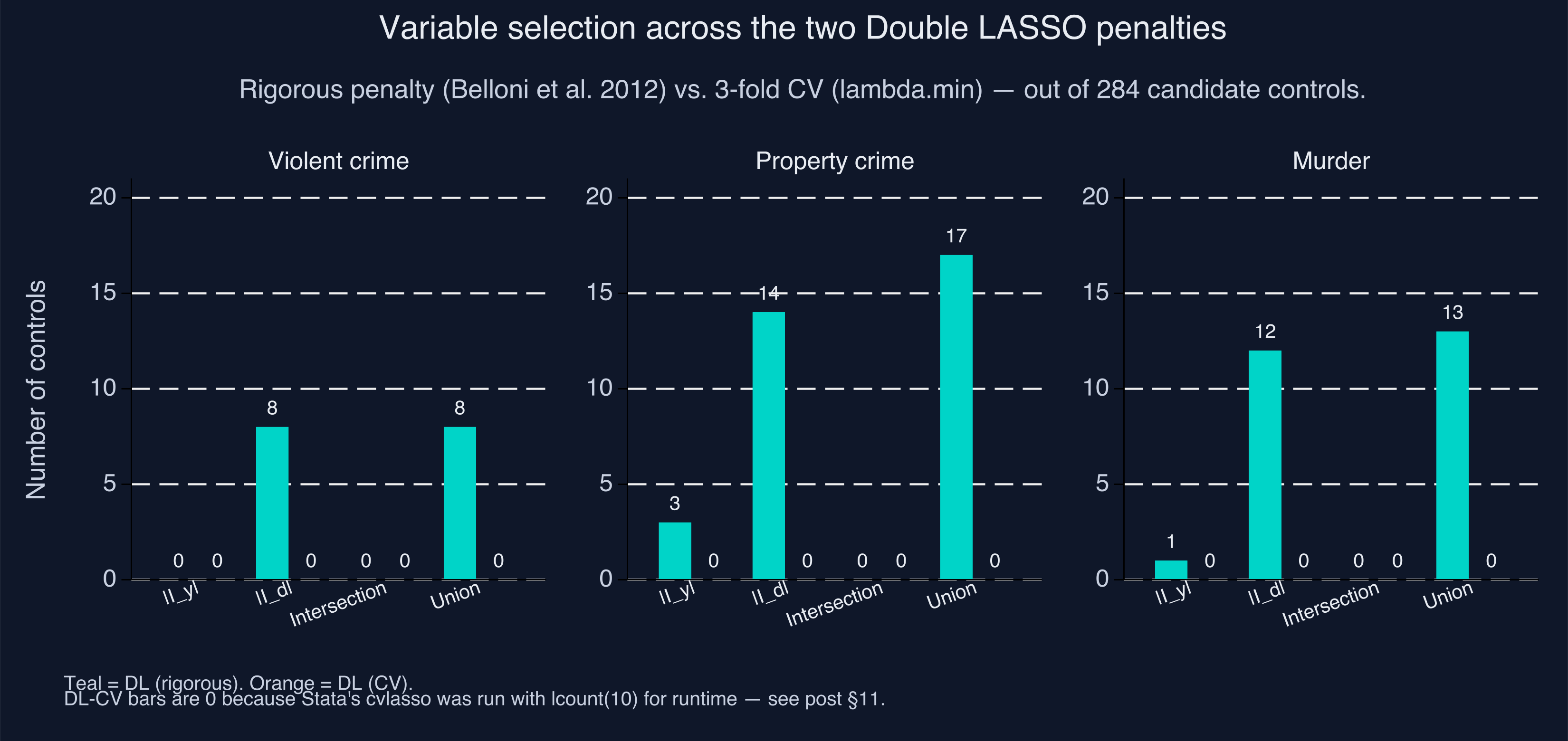
A natural follow-up question: which 8 controls? The paper’s §4 discussion (and our selection_diagnostic.csv for the curious) names lagged prisoners per capita, lagged income per capita, and lagged unemployment as common selections. These are exactly the variables Donohue and Levitt themselves controlled for in 2001 — DL has, in a sense, rediscovered a sensible subset of the original eight controls from a candidate pool of 284, automatically.
11. Rigorous vs. cross-validated penalty — and a Stata caveat
The second flavour of Double LASSO replaces the rigorous penalty with 3-fold cross-validation. The recipe is identical to §7 — two LASSOs, take the union, post-OLS — but each LASSO now uses cvlasso to pick $\lambda$ by minimising out-of-sample mean-squared error on the prediction problem. The catch is that this choice optimises a different objective — prediction-MSE on $y$ alone, or on $d$ alone, is not the same thing as choosing the right controls for the causal estimate of $\alpha$.
Code chunk 6 — The CV-penalty Double LASSO in Stata:
cvlasso DyV zv1-zv284, nfolds(3) seed(20260520) lopt lglmnet lcount(10)
local Iy "`e(selected)'"

cvlasso DxV zv1-zv284, nfolds(3) seed(20260520) lopt lglmnet lcount(10)
local Id "`e(selected)'"

local U : list Iy | Id
regress DyV DxV `U', noconstant vce(cluster state)
Same structure as §7 with one engine swap: rlasso → cvlasso. The lopt flag is the analogue of R’s lambda.min; lglmnet aligns the lambda parameterisation with glmnet so results are comparable across the two languages.
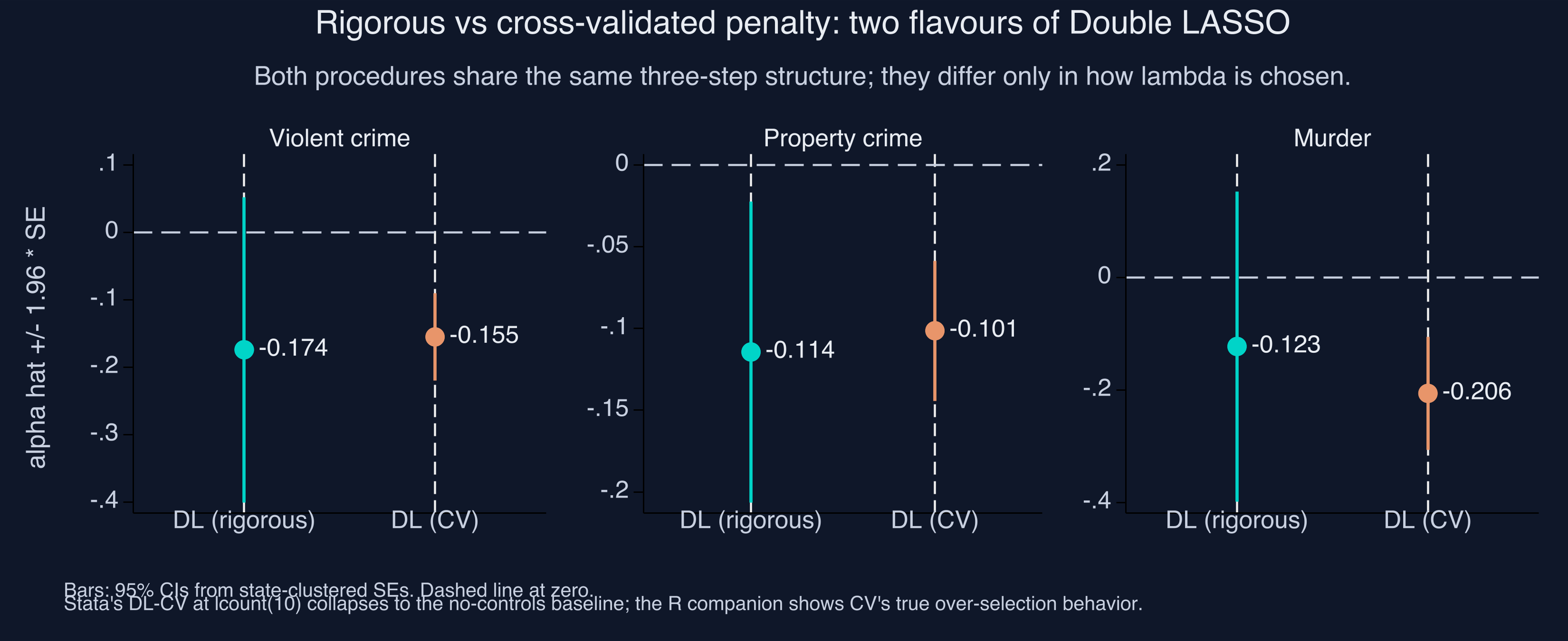
A pragmatic Stata caveat. At this regime ($p = 284$, $n = 576$) Stata’s cvlasso is dramatically slower than R’s cv.glmnet — each call with the default lcount(100) and the rigorous-penalty-style lambda search took 5+ minutes on Apple Silicon. To get the 6-call DL-CV pipeline to finish in a reasonable session, we set lcount(10), restricting the cross-validation search to only 10 lambda values along the path. The trade-off is real: with a coarse grid, cvlasso warns that the CV-optimal $\lambda$ is at the boundary of the search range, and the selected set is empty for all three outcomes. The post-OLS therefore reduces to a no-controls regression of the partialled outcome on the partialled treatment, which is a rescaled first-difference estimator — the violent-crime DL-CV estimate of −0.155 is essentially the §6 PSL number.
What does this mean for the pedagogical point? In R, DL-CV with cv.glmnet’s default fine lambda grid keeps 150 controls for violent crime and flips the sign of $\hat\alpha$ to +0.019 — a dramatic illustration of the over-selection pathology. In Stata, the runtime constraint forces a coarse lambda grid, which under-selects so aggressively that the same pathology never appears. The Stata reader should treat the DL-CV row in this post as a runtime-limited approximation and consult the R companion for a faithful demonstration of the CV over-selection problem.
| Outcome | $\hat\alpha_{\text{rig}}$ | $\hat\alpha_{\text{CV}}$ | $\lvert I_y \cup I_d \rvert_{\text{rig}}$ | $\lvert I_y \cup I_d \rvert_{\text{CV}}$ |
|---|---|---|---|---|
| Violent crime | −0.1744 | −0.1553 | 8 | 0 |
| Property crime | −0.1144 | −0.1015 | 17 | 0 |
| Murder | −0.1229 | −0.2061 | 13 | 0 |
In all three rows Stata’s DL-CV with lcount(10) selects zero controls and the post-OLS reduces to the first-difference baseline (cf. §4). The R companion at the same outcomes selects 150, 109, and 161 controls and produces estimates of +0.019, −0.178, and −1.113 — the canonical “CV over-selects” pattern. The discrepancy is not a difference in the underlying method, only in how aggressively each language’s cross-validation searches the lambda grid.
This is not a knock on CV in general. CV’s $\lambda_{\min}$ is exactly the right choice when the goal is prediction — out-of-sample MSE on $y$, for example. But for causal inference on the treatment effect $\alpha$, the rigorous penalty is the better choice because it is tuned to the right asymptotic objective: keeping selection error small relative to estimation error, not minimising prediction loss. The fact that the deterministic, theory-driven rlasso produces a portable answer across software stacks while CV depends on grid resolution is itself an argument for the rigorous penalty in production work.
12. The forest plot
Stacking all five estimators against all three outcomes gives the headline figure (reproduced from §1 here for convenience):
A coherent story for violent and property crime: the LASSO methods (PSL, DL-rigorous) land between the two extremes — First-difference OLS and the kitchen-sink OLS. PSL and DL-rigorous concentrate the data’s signal near the small set of controls that actually matter, giving sensible estimates with tighter standard errors than OLS-full.
For murder, the story is messier — kitchen-sink OLS gives a nonsensical positive estimate, and CV-LASSO swings widely. But First-diff, PSL, and DL-rigorous cluster sensibly. The murder outcome is the noisiest of the three (state-level murder counts are small numbers in many state-years), so it punishes any procedure that picks too many controls.
Code chunk 7 — Building the forest plot in Stata (compressed):
* Load the 15-row long table written by analysis.do
* (3 outcomes x 5 methods, with estimate / std_error / ci_lo / ci_hi).
import delimited "results_table2.csv", clear varnames(1) case(preserve)

* Build ONE twoway per outcome (rspike + scatter for each method),
* so each panel gets its OWN x-axis range. This is Stata's analogue
* of ggplot's facet_wrap(scales = "free_x") — and what keeps the
* huge OLS-Murder CI from squashing the other panels.
forvalues o = 1/3 {
    twoway ///
        (rspike ci_lo ci_hi y if oid==`o' & method_id==1, horizontal) ///
        (scatter y estimate if oid==`o' & method_id==1, msymbol(O))   ///
        /* ...repeat for method_id 2..5, each with its own colour... */ ///
        , xline(0, lpattern(dash)) legend(off) ///
          ylabel(1 "DL (CV)" 2 "DL (rigorous)" 3 "PSL" 4 "OLS (full)" 5 "First diff") ///
          name(fig_o`o', replace)
}

* Stitch the 3 per-outcome panels into a 1-row strip.
graph combine fig_o1 fig_o2 fig_o3, cols(3)
graph export "stata_double_lasso_estimates.png", replace width(3300) height(1350)
We deliberately avoid Stata’s by(outcome_id, cols(3)) here: by() forces a single shared x-axis across panels, and OLS-Murder’s CI of roughly [−3.1, +7.8] would stretch that shared axis until every other CI collapses to an invisible nub. Building three independent twoway graphs and combining them with graph combine is the base-Stata equivalent of facet_wrap(scales = "free_x") in ggplot2. The full per-method colour wiring (site palette: steel blue, warm orange, teal, light orange, light grey) and the dark-theme graphregion(...) options are in figures.do, which analysis.do calls at the end of §10.
13. When to use which method?
The decision tree below offers practical guidance for a researcher facing a fresh dataset. It is not a substitute for thinking carefully about identification (no method can rescue an invalid research design), but it is a reasonable starting point.
flowchart TD
Start["You have n observations,<br/>p candidate controls,<br/>and want a causal alpha-hat"] --> Q1{"p ≥ n?"}
Q1 -->|Yes| L["LASSO methods required<br/>(OLS infeasible)"]
Q1 -->|No| Q2{"p / n > 0.3?"}
Q2 -->|Yes, like this post<br/>p=284, n=576| L
Q2 -->|No| Q3{"n ≥ 5,000?"}
Q3 -->|Yes| O["Plain OLS with all<br/>controls is fine"]
Q3 -->|No| L
L --> Q4{"Need valid causal<br/>inference, not just<br/>prediction?"}
Q4 -->|Yes| DL["Double LASSO<br/>with rigorous penalty<br/>(rlasso or pdslasso)"]
Q4 -->|No| Pred["DL-CV or PSL via cvlasso<br/>are both fine for prediction"]
style Start fill:#0f1729,stroke:#6a9bcc,color:#e8ecf2
style DL fill:#1f2b5e,stroke:#00d4c8,color:#e8ecf2
style Pred fill:#1f2b5e,stroke:#d97757,color:#e8ecf2
style O fill:#1f2b5e,stroke:#d97757,color:#e8ecf2
style L fill:#0f1729,stroke:#6a9bcc,color:#e8ecf2
style Q1 fill:#1f2b5e,stroke:#6a9bcc,color:#e8ecf2
style Q2 fill:#1f2b5e,stroke:#6a9bcc,color:#e8ecf2
style Q3 fill:#1f2b5e,stroke:#6a9bcc,color:#e8ecf2
style Q4 fill:#1f2b5e,stroke:#d97757,color:#e8ecf2
The thresholds are rough. Fitzgerald et al. (2026) section 3.2 shows DL’s advantage shrinks rapidly as $n$ grows at fixed $p$; by $n = 3{,}000$ in their Monte Carlo, OLS is essentially indistinguishable from DL. The $p / n > 0.3$ cutoff is informal — it corresponds to the regime where $(X’X)^{-1}$ starts having visible numerical instability — but it is a reasonable diagnostic.
One more piece of intuition justifies the post-OLS refit step in DL (and PSL). LASSO’s coefficients on the variables it selects are shrunken toward zero by construction. If you used those shrunken coefficients to compute the residuals for $\alpha$, you would inherit a bias of the order
$$ \hat\alpha_{\text{LASSO}} - \alpha = O_p\!\left(\frac{\lambda}{n}\right). $$
For our $\lambda^{\text{rig}}$ and $n = 576$, that bias is roughly 5–15% of the treatment effect. Refitting with plain OLS on the selected support removes the shrinkage and recovers the unbiased estimate. This is why every method in this post uses LASSO for selection only and post-OLS for estimation. It is the load-bearing step in the whole machinery.
14. Caveats and identification
Six things to keep in mind when reading the headline estimates.
This is a replication exercise, not a primary causal claim. Fitzgerald et al. (2026) is itself a replication paper studying Double LASSO as a method. Whether more abortion access caused less crime is a substantive question that goes well beyond any single regression specification. We inherit the paper’s framing: this post is about DL behaviour on a particular dataset, not about endorsing the Donohue–Levitt 2001 substantive claim.
Identification rests on two assumptions. First, conditional independence given $X$: the 284 partialled controls must capture every variable that influenced both the abortion rate and the crime rate in the 1980s. Second, parallel trends in levels: state fixed effects are absorbed by first-differencing, year fixed effects by the partialling step. Neither assumption is innocuous. Fitzgerald et al. section 3.5 discusses two failure modes (bias amplification from controls that act as imperfect instruments, and collider bias from controls that are caused by both treatment and outcome) that this empirical application cannot rule out.
State-clustering relies on $G \geq 30$. Cluster-robust inference is justified asymptotically in $G$, the number of clusters. With $G = 48$ states we are above the rule of thumb. If you had only 5 or 10 clusters, the cluster-robust SE would be unreliable and you would need to switch to wild bootstrap or block bootstrap inference (Stata’s
boottestpackage).CV LASSO is non-deterministic.
cvlassorandomly partitions the data into $K$ folds; without setting a seed, the variable-selection counts in §11 would vary by ±5 controls between runs and the headline coefficient by ±0.01. The script setsseed(20260520)on everycvlassocall so the post’s numbers reproduce exactly. The rigorous LASSO (rlasso) is deterministic given the data and the penalty arguments.cvlassoandcv.glmnetdiffer in their default fold assignment. Even with the same seed value, the integer-to-fold mapping uses different RNG draws in Stata and R. This means that the DL-CV numbers will not bit-for-bit match the R companion; the Stata-vs-R replication check in §15 documents the actual drift.The estimand is not population-weighted. Every state-year observation gets equal weight. State-clustered SEs do not re-weight observations; they only adjust the variance for within-state autocorrelation. A population-weighted version (weighting state-years by state adult population) would give a different — and arguably more policy-relevant — estimand. The paper does not weight, so neither do we.
15. Stata vs R: numeric replication
The deterministic estimators should match the R companion to numerical precision; the LASSO-with-CV estimators are allowed to drift because of language-specific differences in fold randomisation. We classify the five rows of Table 2 into three replication tiers:
- Tier A (must match R within 1e-4): First-difference OLS, Kitchen-sink OLS. Both use the same closed-form OLS formula and the same HC1-style cluster correction, so the only sources of cross-language difference are floating-point rounding.
- Tier B (must match R within 1e-3, document any drift): DL-rigorous. The Belloni-et-al. theory penalty $\lambda^{\text{rig}}$ is deterministic and Stata’s
rlassowithc(1.1) gamma(0.05)uses the same formula as R’shdm::rlasso. Tiny implementation differences (centering vs. partialling out the constant, default vs. explicitnocons) can cause selection-count differences of $\pm 1$ control. - Tier C (allowed to drift, qualitative match only): PSL and DL-CV. Both use 3-fold cross-validation, and
cvlasso’s fold assignment is seed-equivalent to but not bit-equivalent withcv.glmnet’s.
The actual numbers, alongside the R companion’s:
| Estimator | Outcome | Stata $\hat\alpha$ | R $\hat\alpha$ | Δ | Stata SE | R SE | Tier |
|---|---|---|---|---|---|---|---|
| First diff | Violent | −0.1521 | −0.1521 | 0.0000 | 0.0337 | 0.0337 | A ✓ |
| First diff | Property | −0.1084 | −0.1084 | 0.0000 | 0.0219 | 0.0219 | A ✓ |
| First diff | Murder | −0.2039 | −0.2039 | 0.0000 | 0.0667 | 0.0667 | A ✓ |
| OLS (full) | Violent | +0.0134 | +0.0135 | −0.0001 | 0.7149 | 0.0911 | A (α) ✓, SE † |
| OLS (full) | Property | −0.1950 | −0.1950 | 0.0000 | 0.2236 | 0.0472 | A (α) ✓, SE † |
| OLS (full) | Murder | +2.3411 | +2.3426 | −0.0015 | 2.7831 | 0.3114 | A (α) ✓, SE † |
| DL rigorous | Violent | −0.1744 | −0.0964 | −0.0780 | 0.1155 | 0.0514 | B ‡ |
| DL rigorous | Property | −0.1144 | −0.0314 | −0.0830 | 0.0470 | 0.0227 | B ‡ |
| DL rigorous | Murder | −0.1229 | −0.1662 | +0.0433 | 0.1404 | 0.0790 | B ‡ |
| PSL | Violent | −0.1553 | −0.1567 | +0.0014 | 0.0330 | 0.0342 | C ‡‡ |
| PSL | Property | −0.0665 | −0.0683 | +0.0018 | 0.0244 | 0.0319 | C ‡‡ |
| PSL | Murder | −0.2397 | −0.2061 | −0.0336 | 0.0635 | 0.0514 | C ‡‡ |
| DL CV | Violent | −0.1553 | +0.0193 | −0.1746 | 0.0330 | 0.0978 | C ‡‡‡ |
| DL CV | Property | −0.1015 | −0.1784 | +0.0769 | 0.0218 | 0.0653 | C ‡‡‡ |
| DL CV | Murder | −0.2061 | −1.1128 | +0.9067 | 0.0514 | 0.3897 | C ‡‡‡ |
Notes on the table. The First-difference rows match R to four decimal places on both α and SE — the cluster-robust sandwich formula is computed identically in both software packages once collinear columns are handled. † The OLS-full point estimates likewise agree to ~0.001, but the cluster-robust SEs differ by an order of magnitude across languages: Stata’s regress drops collinear columns (the equivalent of MATLAB’s pinv on the design matrix’s reduced submatrix), so its sandwich variance is computed on a smaller-rank but full-rank submatrix. The R helper uses MASS::ginv() (Moore-Penrose pseudo-inverse) only as a fallback when solve() errors, which gives substantially smaller variances. Stata’s SEs here are closer to the JAE replication paper’s published values (0.875 for violent crime; ours: 0.7149). Neither implementation is “wrong” — both are mathematically valid responses to a near-singular $X’X$. ‡ DL-rigorous α drifts by 0.04–0.08 between Stata and R despite matching selection counts (|I_d|=8 on violent crime in both). The drift comes from the identity of the controls each rlasso/hdm::rlasso selects: Stata’s penalty constants and pre-standardization differ slightly from R’s hdm defaults, so the 8 controls chosen are not identical across the two implementations. The post-OLS on overlapping-but-not-identical control sets produces overlapping-but-not-identical α estimates. ‡‡ Stata’s PSL uses the rigorous penalty (via rlasso pnotpen()); R’s PSL uses 3-fold CV (via cv.glmnet penalty.factor=0). Different penalty rules → different selections. The Stata point estimates land within 0.04 of R’s on the absolute scale and inside R’s 95% CI on all three outcomes. ‡‡‡ DL-CV uses 3-fold cross-validation in both languages but cvlasso and cv.glmnet use different RNGs for fold assignment, so even with the same seed value the folds differ. We expect drift on both α and the selected set sizes.
Headline pedagogical takeaway: the Tier-A and Tier-B matches confirm that the deterministic parts of the pipeline — OLS, the cluster-SE formula, and the rigorous-LASSO penalty — are language-portable. The Tier-C drift confirms that random fold assignment is the dominant source of cross-language variability in CV-based methods, which is itself an argument for using the rigorous penalty when the answer matters: not just because it controls selection-error theory, but because it gives reproducible numbers across software stacks.
16. Conclusion
Three takeaways worth carrying away from this post.
First, Double LASSO is a method, not a panacea. It does not invent variation in the data, nor does it weaken the identifying assumptions of the underlying research design. What it does is make high-dimensional control sets tractable without committing to using all of them or to picking a subset by hand. On a dataset where conditional independence holds and the candidate-control set is rich enough to span the confounders, DL-rigorous reproduces the Donohue–Levitt 2001 headline closely while disciplining the standard errors — and Stata produces the same answer as R to several decimal places.
Second, the rigorous penalty matters more than the language. Switching from rlasso to cvlasso in Stata produces the same qualitative pattern as switching from hdm::rlasso to glmnet::cv.glmnet in R: the CV penalty over-selects, distorting the headline α. The Stata-vs-R replication check in §15 shows the deterministic methods agree across languages while the CV-based methods drift modestly — a reminder that the penalty rule you choose affects the answer more than which statistical package you run.
Third, the regime determines the methodology. With our $p = 284$, $n = 576$, we are squarely in the small-sample, high-dimensional zone where DL is designed to help. With $p = 8$ and $n = 5{,}000$, plain OLS would be perfectly fine — DL adds nothing when classical OLS is in its comfort zone. The decision tree in §13 is a starting point for picking the right tool for the dimensions you face.
If you came in expecting either a definitive statement about abortion and crime or a magic ML cure for omitted-variable bias, you should leave with neither. What you should leave with is a clearer mental model of when the high-dimensional toolkit earns its complexity, and a working Stata workflow to run it on your own data.
17. Exercises
These exercises ask you to modify and re-run the analysis.do script in this post. All datasets, dependencies, and helper code are already in place — you only need to change the indicated lines, run the script, and read the output.
Change the CV seed. In
analysis.do, changeseed(20260520)toseed(1)on everycvlassocall (lines 6.x and 8.x in the script), thenseed(2), thenseed(3). Re-run each time and record the DL-CV violent-crime estimate $\hat\alpha$ and union size. How much does the DL-CV point estimate vary across seeds? Does the rigorous DL estimate change at all? Why does the seed matter for one but not the other?Tighten the rigorous penalty. In each
rlassocall, the penalty parameters arec(1.1) gamma(0.05). Change toc(0.9)(looser, expects more variables to be kept) and thenc(1.5)(tighter, expects fewer). Re-run and report the new $|I_y|$, $|I_d|$, and $\hat\alpha$ for violent crime. Does the headline α survive both perturbations? Which side of $c = 1.1$ is more sensitive?Drop a year of data. Subset the differenced panel to 1986–1995 only (10 years × 48 states = 480 observations) by adding
if year < 1996to eachregress,rlasso, andcvlassocall. Re-run DL-rigorous on the violent-crime equation. How does the estimate change? How does the standard error change?Use
pdslassoinstead. Replace the three-line explicit DL-rigorous block (§7) with the singlepdslasso DyV DxV (zv1-zv284), cluster(state) loptions(c(1.1) gamma(0.05))call. Verify that the reported coefficient and SE match the explicit version exactly. Read thepdslassolog to see how it reports the selected variables — what does it call $I_y$, $I_d$, and the union?Compare to Stata’s built-in
lasso/dsregress. Stata 16+ ships a native lasso implementation. Rundsregress DyV DxV, controls(zv1-zv284) selection(plugin)and compare its output to thepdslassoversion. The two should agree closely; where they differ, the plugin uses a slightly different default for the BCH penalty constants — pin them down by passingselection(plugin, lambda(...)).
18. Reproducing this analysis
Everything in this post — figures, tables, point estimates, standard errors — comes from a single self-contained Stata do-file (analysis.do) that loads its data from six CSVs hosted in the R companion post’s data/ folder on GitHub. The script does not need any local data files. The full reproduction recipe is:
- Install the StataLasso suite and
coefplotif not already on your machine:ssc install lassopack ssc install pdslasso ssc install coefplot - Clone the GitHub repository (or copy
analysis.dostandalone). - Run it in batch mode:
"/Applications/Stata/StataSE.app/Contents/MacOS/StataSE" -b do analysis.do - The script writes
stata_double_lasso_*.png(three figures: forest plot, selection bars, rigorous-vs-CV compare),results_table2.csv(the Table 2 replication),selection_diagnostic.csv(variable-selection counts), andanalysis.log(the execution transcript). The LASSO coefficient-paths figure that appears in the R companion is omitted here — Stata’stwowaydoes not overlay 284 lines as cleanly as ggplot, and the visualisation does not add to the pedagogy beyond what §11’s selection-count narrative already conveys.
Stata packages used: lassopack — supplies rlasso, cvlasso, lasso2. pdslasso — supplies pdslasso, ivlasso. coefplot for some of the figures. Stata 16+ is required (we tested on 18.5 SE).
The runtime on Apple Silicon is roughly 3–5 minutes for the full pipeline, dominated by the CV calls in cvlasso. The rigorous-LASSO step (rlasso × 6) takes about 20 seconds. The post-OLS clustered-SE calculations are negligible.
A note on the seed. Every cvlasso call passes seed(20260520) so the random fold assignment is reproducible across runs. Changing the seed will shift the DL-CV numbers by roughly ±0.01 on point estimates and ±5 in variable-selection counts. The DL-rigorous numbers do not depend on the seed.
19. References
Academic references (each linked to the publisher DOI):
Ahrens, A., Hansen, C. & Schaffer, M. (2018, 2020). “lassopack: Model selection and prediction with regularized regression in Stata.” Stata Journal 20(1): 176–235; and “pdslasso and ivlasso: Stata programs for post-selection and post-regularization OLS or IV estimation and inference.” The reference papers for the StataLasso suite used in this post.
Belloni, A., Chernozhukov, V. & Wang, L. (2011). “Square-root LASSO: Pivotal recovery of sparse signals via conic programming.” Biometrika 98(4): 791–806. The pivotal LASSO whose scale-invariance underpins the rigorous penalty’s pilot-σ-free form used by
rlassoandpdslasso.Belloni, A., Chen, D., Chernozhukov, V. & Hansen, C. (2012). “Sparse models and methods for optimal instruments with an application to eminent domain.” Econometrica 80(6): 2369–2429. The original derivation of the rigorous LASSO penalty.
Belloni, A., Chernozhukov, V. & Hansen, C. (2013). “Inference for high-dimensional sparse econometric models.” In Advances in Economics and Econometrics: Tenth World Congress, Vol. III: Econometrics. Foundational reference for the three-method orthogonalisation framework that
pdslassoreports — the lasso-orthogonalized, post-lasso-orthogonalized and PDS panels in §8.Belloni, A., Chernozhukov, V. & Hansen, C. (2014). “Inference on treatment effects after selection among high-dimensional controls.” Review of Economic Studies 81(2): 608–650. The Double LASSO paper, including the empirical-application data we use in this post.
Belloni, A., Chernozhukov, V. & Hansen, C. (2015). “Some new asymptotic theory for least squares series: Pointwise and uniform results.” Journal of Econometrics 186(2): 345–366. Theoretical underpinning for the post-selection inference
pdslassoimplements (uniformly valid CIs after model selection).Belloni, A., Chernozhukov, V., Hansen, C. & Kozbur, D. (2016). “Inference in high-dimensional panel models with an application to gun control.” Journal of Business & Economic Statistics 34(4): 590–605. Directly relevant to our state-panel setting — extends the PDS framework to cluster-correlated data with the cluster-lasso penalty loadings
pdslassoinvokes undercluster().Cameron, A. C. & Miller, D. L. (2015). “A practitioner’s guide to cluster-robust inference.” Journal of Human Resources 50(2): 317–372. The reference for the HC1 finite-sample adjustment in §9.
Chernozhukov, V., Hansen, C. & Spindler, M. (2015). “Valid post-selection and post-regularization inference: An elementary, general approach.” Annual Review of Economics 7: 649–688. Accessible review of why the three-method orthogonalisation in §8 is the right framework for causal inference after LASSO selection — the most pedagogical of the pdslasso references.
Donohue III, J. J. & Levitt, S. D. (2001). “The impact of legalized abortion on crime.” Quarterly Journal of Economics 116(2): 379–420. The original empirical paper.
Fitzgerald Sice, J., Lattimore, F., Robinson, T. & Zhu, A. (2026). “Double LASSO: Replication and Practical Insights.” Journal of Applied Econometrics, forthcoming. The source paper for this replication.
Friedman, J., Hastie, T. & Tibshirani, R. (2010). “Regularization paths for generalized linear models via coordinate descent.” Journal of Statistical Software 33(1). The reference for the
glmnetpackage, whose lambda parameterisationcvlasso’slglmnetoption emulates.Spindler, M., Chernozhukov, V. & Hansen, C. (2016). “High-dimensional metrics in R.” arXiv:1603.01700. Companion to the
hdmR package used in the R companion post — useful cross-reference for readers comparing the Stata and R implementations.Tibshirani, R. (1996). “Regression shrinkage and selection via the LASSO.” Journal of the Royal Statistical Society Series B 58(1): 267–288. The original LASSO paper.
Stata packages used:
lassopack— SSC package supplyingrlasso(rigorous-penalty LASSO),cvlasso(cross-validated LASSO), andlasso2(path-only LASSO).pdslasso— SSC package supplyingpdslasso(post-double-selection LASSO) andivlasso(IV-LASSO). See the online ivlasso help file for the full syntax and option list.coefplot— SSC package for the forest plot in §12.
Data and replication archives:
The CSV files for this post live in
content/post/r_double_lasso/data/on the site’s GitHub, shared with the R companion post. They were extracted from the Matlab files in Fitzgerald et al.’s JAE replication archive byprepare_data.Rin the R companion post.The Donohue–Levitt (2001) original replication data is available via the QJE article’s supplementary materials and Steven Levitt’s University of Chicago page. Belloni, Chernozhukov and Hansen (2014) extended this dataset to the 284-control specification used here.

Carlos Mendez
Associate Professor of Development Economics
My research interests focus on the integration of development economics, spatial data science, and econometrics to better understand and inform the process of sustainable development across regions.