Visualizing Regression with the FWL Theorem in Stata

What ‘controlling for’ looks like as a scatter plot

−0.093naive slope · wrong sign

+0.212after partialling out income

0.212288manual FWL matches to 6 decimals

Carlos Mendez

Nagoya University (GSID)

September 28, 2026

The Tension

Act I

“Controlling for income” is the one move you can never draw on a scatter

A store manager asks: do coupons lift sales? The raw scatter says no — more coupons, lower sales.

“Holding income fixed” lives in three dimensions. How do you put that on two axes?

This is the hook of the whole tutorial. Everyone uses the phrase “controlling for X,” but almost no one can point to the picture. The FWL theorem is the bridge — it turns a multidimensional regression coefficient into a two-dimensional slope you can literally plot. Keep this concrete: one manager, one question, one scatter.

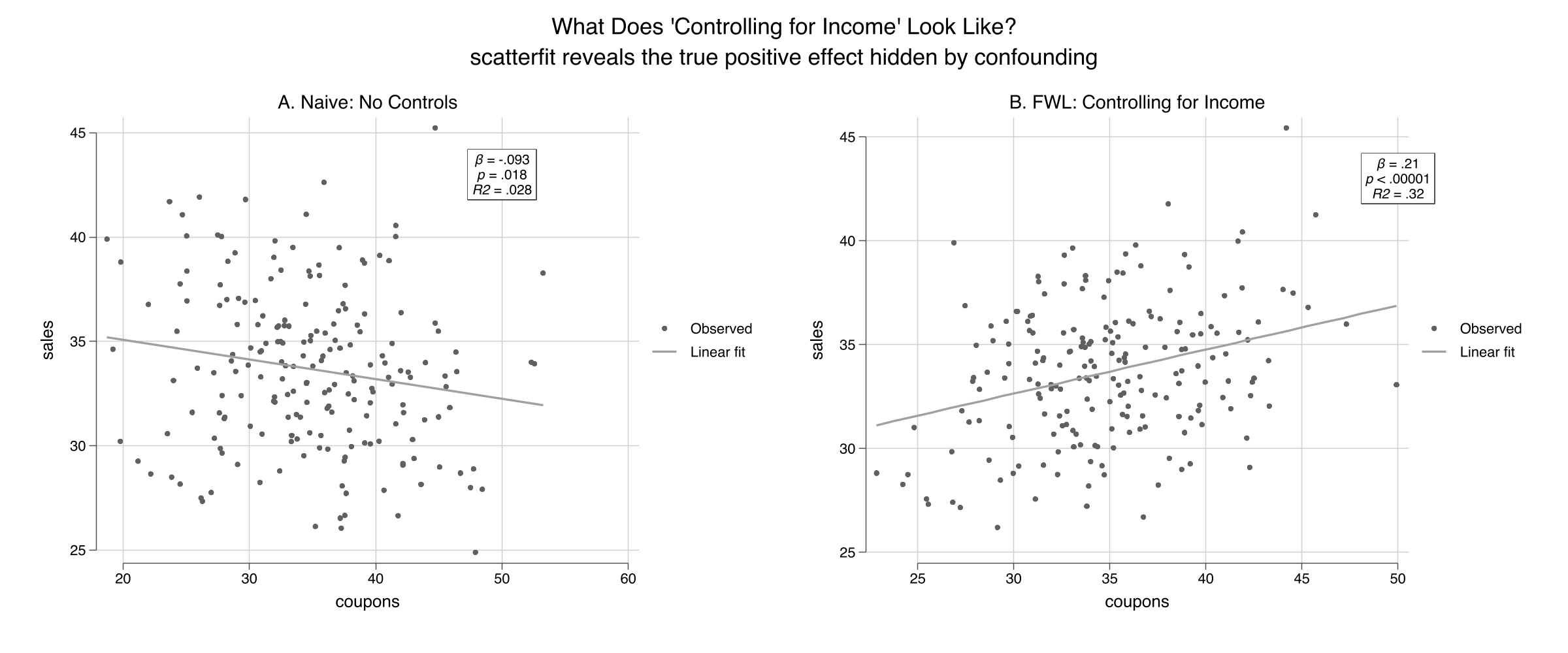
Same data, opposite slopes — one picture is honest and one is a lie

Naive scatter (left): negative slope, R² = 0.028. After controls(income) the slope reverses to positive, R² = 0.32. Same 200 stores, two pictures.

Spoiler figure — don’t explain the mechanism yet. Just plant that the left and right panels are the same dataset, and the slope flips sign. The left panel is the naive scatter everyone draws; the right is what FWL lets you see. We earn the right panel in Act II.

Where we’re going

• A confounded toy dataset where the right answer is known
• scatterfit — partialling-out in one command
• The same number by hand, to six decimals (the FWL identity)
• Fixed effects as FWL on group dummies — flights and a wage panel

The Investigation

Act II

A toy dataset built so income confounds the coupon–sales link

• Outcome — store sales (200 stores)
• Treatment — coupons distributed (true effect +0.2)
• Confounder — income: rich areas get fewer coupons but buy more

Coupons and income are negatively linked (−0.71) — a backdoor the naive slope misses.

The store targets promotions at lower-income areas, so coupons and income are negatively linked (−0.71). Income also lifts sales. That opens a backdoor path the naive slope never blocks. The data-generating process is known: coupons → sales is +0.2, income → coupons is −0.5, income → sales is +0.3. Because we built it, we know the naive estimate is wrong on purpose. This is the controlled lab where we can check that FWL recovers the truth.

The raw correlation lies: coupons and sales correlate −0.17

Pair	Correlation	Reading
coupons · sales	−0.17	looks like coupons hurt sales
income · coupons	−0.71	store sends fewer coupons to rich areas
income · sales	+0.50	rich areas buy more

The true coupon effect is +0.2 — the negative raw correlation is income leaking through.

Walk the three rows. The first row is the trap. Rows two and three explain why: income is the hidden third variable correlated with both. Any tool that ignores income inherits this leak. That motivates partialling out.

The FWL theorem: residualize first, then read one slope

\[\hat\beta_1=\frac{\operatorname{Cov}(\tilde y,\tilde x_1)}{\operatorname{Var}(\tilde x_1)}\]

Residualize both axes on \(Z\), then read one slope — it equals the multiple-regression coefficient on \(x_1\).

The tildes mean “the part \(Z\) cannot explain.” Two paths, one number.

Spell out the recipe aloud: regress \(y\) on the controls \(Z\) and keep the residual \(\tilde y\); regress \(x_1\) on \(Z\) and keep \(\tilde x_1\); the simple slope of \(\tilde y\) on \(\tilde x_1\) is the multiple-regression coefficient on \(x_1\). This is the algebraic heart of the deck. The multivariate β₁ is not an approximation of the residual-on-residual slope — it is exactly that slope. Frisch & Waugh (1933) and Lovell (1963) proved it. Everything downstream — scatterfit, reghdfe, fixed effects — is this identity in disguise.

One option turns the multiple regression into a partial-regression plot

scatterfit sales coupons, regparameters(coef pval r2)              // naive: −0.093
scatterfit sales coupons, controls(income) regparameters(coef pval r2)  // FWL: +0.212

controls(income) tells scatterfit to call reghdfe, residualize both axes on income, then plot \(\tilde y\) against \(\tilde x_1\).

scatterfit (Ahrens 2024) is built on reghdfe. The controls() option does the FWL residualization internally and plots the residuals with a fitted line. The regparameters() option stamps the coefficient, p-value, and R² right on the plot — a feature R’s fwl_plot() and Python’s manual FWL lack.

Partialling out income flips the slope from −0.093 to +0.212

Term	Naive OLS	+ income	Reading
coupons	−0.0934	0.2123	sign reverses
income	—	0.3004	confounder, near true 0.3
R²	0.028	0.321	variation explained jumps

The +0.212 lands right on the true effect of +0.2; income’s coefficient lands on its true 0.3.

This is the payoff of the controls() call as a table. The coupon coefficient goes from −0.093 (significant but wrong-signed) to +0.212. R² climbs from 0.03 to 0.32. The full regression on the right is exactly what the right-hand scatter on the spoiler slide was showing.

The omitted-variable-bias formula predicts the gap exactly

\[\hat\beta_{\text{naive}}=\hat\beta_{\text{full}}+\hat\gamma\,\hat\delta:\qquad -0.0934=0.2123+(-0.3057)\]

\(\hat\gamma=0.3004\) is income’s effect on sales in the full model; \(\hat\delta=-1.0174\) is the slope of income on coupons. Their product is the bias, and it closes the gap exactly.

Nothing mysterious: a positive \(\hat\gamma\) times a negative \(\hat\delta\) drags the naive estimate down.

OVB is the flip side of FWL. γ̂ = 0.3004 is the income coefficient in the full model; δ̂ = −1.0174 is the slope from the auxiliary regression of income ON coupons (regress income coupons) — not coupons on income. Their product, −0.3057, is exactly naive −0.0934 minus controlled 0.2123: an algebraic identity, and the do-file asserts it to 1e-8. In the population δ = −1.0, so the naive slope converges to 0.2 + 0.3 × (−1.0) = −0.10. The point: the confounding is fully accounted for by one product of two slopes.

By hand, the residual-on-residual slope is 0.212288 — six matching decimals

* Step 1 — residualize sales on income
regress sales income
predict resid_sales, residuals
* Step 2 — residualize coupons on income
regress coupons income
predict resid_coupons, residuals
* Step 3 — regress residual on residual
regress resid_sales resid_coupons      // slope = 0.212288

The manual slope 0.212288 equals the full-regression coefficient 0.212288 — not close, identical.

This is the proof-by-doing. Three regress/predict steps reproduce the multivariate coefficient to six decimals. It is an algebraic identity, not a numerical coincidence — which is why scatterfit can draw it as a single fitted line. The intercept on the residual regression is essentially zero, as FWL guarantees.

The residual regression reproduces the coefficient to six decimals

0.212288

Manual FWL slope = full-regression coupon coefficient. Same number, two paths.

The headline of Act II as one giant number. Manual three-step FWL and the one-line multiple regression agree to six decimals. This is the identity made visible — and it is what licenses the partial-regression scatter as a faithful picture of the controlled relationship.

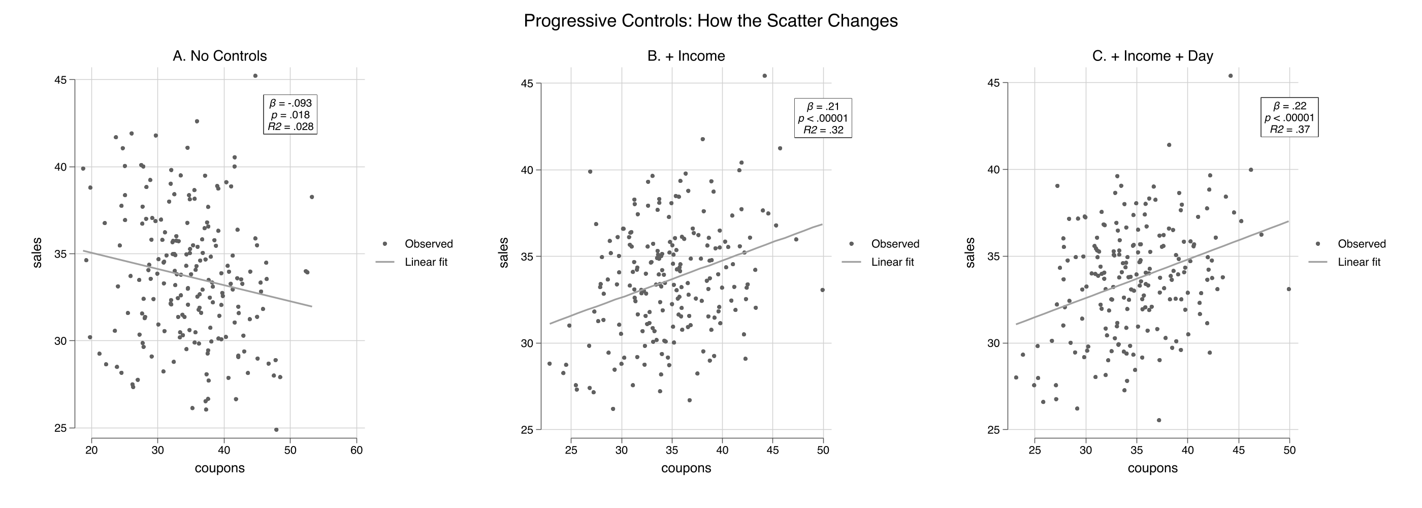
Add controls progressively and watch the scatter tighten

No controls (left, R² = 0.028) → + income (center, R² = 0.32) → + income + day-of-week (right, R² = 0.37). Each panel residualizes on more, so the cloud tightens.

Each panel is the same coupons–sales relationship after partialling out more controls. The coefficient moves −0.093 → +0.212 → +0.222; R² climbs 0.028 → 0.32 → 0.37. The visual story: more controls absorbed means a tighter, more honest cloud. Same FWL machinery, more columns in Z.

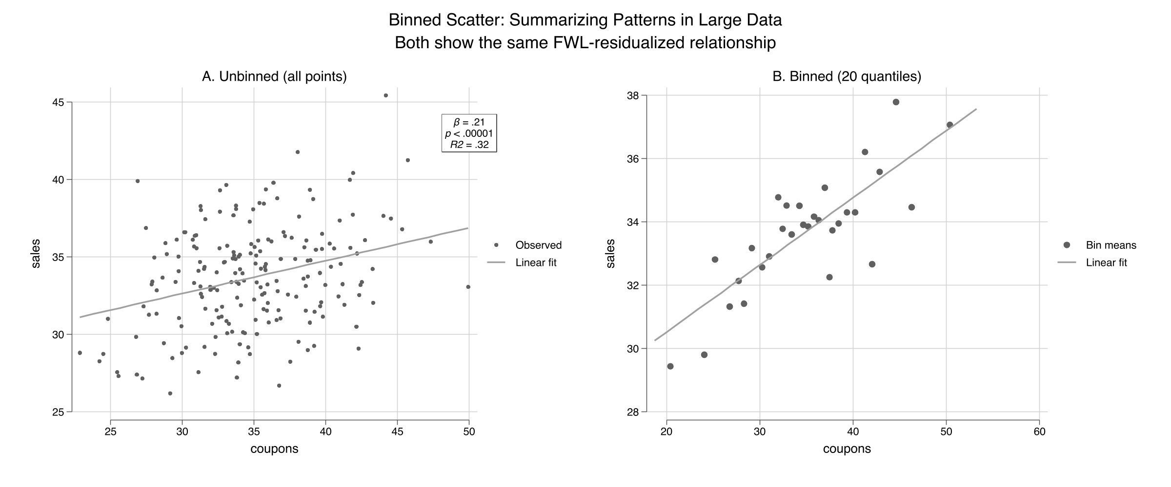
For thousands of points, bin the scatter — the slope is unchanged

Unbinned (left) vs. binned into 20 quantiles (right). Both show the same FWL-residualized fit (β = 0.21, R² = 0.32); binning replaces 200 points with 20 readable means.

With 5,000 or 5 million points a raw scatter is a black blob. The binned option groups x into quantile bins and plots bin means, but the line is still fit on the full data — so the slope is identical. This is one of scatterfit’s edges over R’s fwl_plot and Python’s manual route. For 200 stores the difference is cosmetic; for production data it is essential.

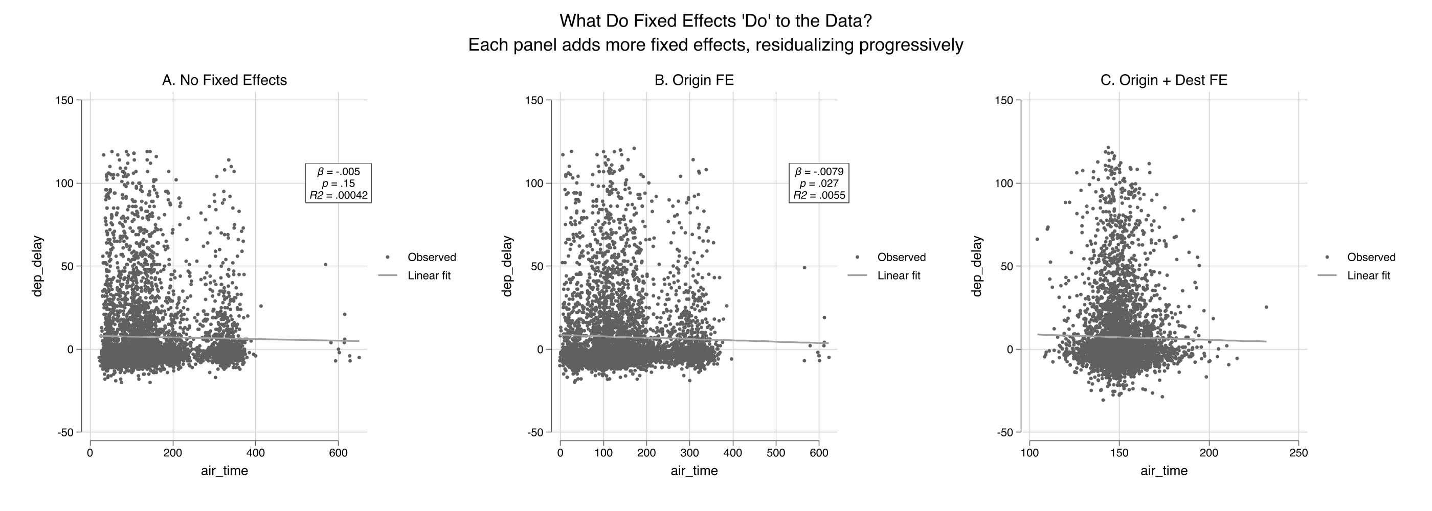
Fixed effects are just FWL on group dummies — and they reshape the cloud

Air-time vs. delay, NYC flights. No FE (left, R² ≈ 0) → origin FE (center) → origin + destination FE (right). fcontrols() demeans by group via reghdfe.

fcontrols() in scatterfit partials out categorical group means — the FWL residualization where Z is a set of dummies. Panel A is the raw cloud; B removes the three origin-airport means; C removes destination means too, leaving deviations from the origin and destination averages. The air-time coefficient moves −0.005 → −0.008 → −0.032 across the panels. These are estimated on the 5,000-flight sample; the R post estimates on all 317,578 cleaned flights and gets −0.003 → −0.006 → −0.007, so do not expect the flights numbers to match across editions. reghdfe does the demeaning internally, which is why it scales to huge data.

The Resolution

Act III

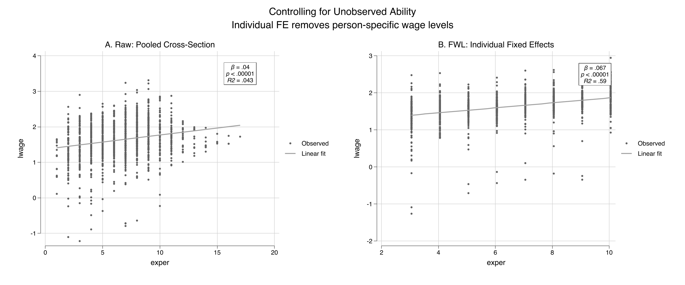
In a wage panel, individual fixed effects lift R² from 0.04 to 0.59

Raw pooled cross-section (left, R² = 0.043) vs. individual fixed-effects residualized scatter (right, R² = 0.59). fcontrols(nr) strips each person’s average — within-person experience returns ≈ 7%.

The Wooldridge wage panel: 545 individuals, 8 years. Panel A’s wide fan is people of the same experience earning very different wages — that spread is unobserved ability. fcontrols(nr) demeans each person against themselves (the within transformation), leaving within-person variation. R² jumps 0.04 → 0.59 and the slope steepens to a ≈7% within-person return to experience. Same FWL algebra, with person dummies as the controls.

One algebra, three languages — only the syntax changes

Stata (scatterfit)

• scatterfit y x — raw
• , controls(z) — partial out Z
• , fcontrols(fe) — group FE
• , binned · regparameters()

R / Python

• R: fwl_plot(y ~ x + z)
• R: fwl_plot(y ~ x | fe)
• Python: manual resid()
• no binning / on-plot stats

R and Stata load the same 200 stores, so their numbers match; Python simulates its own 50 stores, so its numbers differ but obey the same identities.

This is the trilogy payoff. The R and Stata posts load the same store_data.csv (200 stores), so they report the same naive −0.093, controlled +0.212, and OVB −0.3057. The Python post simulates its own 50-store sample from the same data-generating process, so its numbers differ (naive −0.1059, controlled +0.2673) while the FWL and OVB identities hold exactly there too. Stata’s extras (binned scatters, on-plot regparameters) are conveniences, not different math. A student who learns FWL once can read it in any language.

Does the scatter make this causal? No — it only makes the algebra visible

Objection. A partial-regression plot looks like proof that coupons cause +0.212.

Response. It is not. FWL is an algebraic identity — it visualizes “holding Z fixed,” nothing more. The +0.212 is causal here only because we built the DGP.

In real data, identification still rests on having the right controls in Z. FWL shows what a coefficient is, not whether it deserves a causal reading. Steelman, don’t strawman. The partial-regression plot is seductive — it looks like causal evidence. But it is purely mechanical: it reports the slope of the multiple regression, full stop. Whether that slope is the causal effect depends entirely on whether Z blocks the relevant backdoors. In the toy data it does (we wrote the DGP); in the wild, that is an assumption, not a guarantee.

“Controlling for X” is a residual-on-residual slope you can finally draw.

The single sentence to leave them with. FWL turns the abstract phrase “controlling for income” into a concrete picture: residualize both axes, plot, read one slope. The coefficient you would have reported from a multiple regression is exactly that line — −0.093 became +0.212, and you can see why.