IV Estimation with Panel Data

Economic shocks and civil conflict across 5,689 African regions

−0.2962SLS effect of lights on conflict

0.001OLS estimate · attenuated to zero

40.3first-stage F · instruments are strong

Carlos Mendez

Nagoya University (GSID)

June 11, 2026

The Tension

Act I

Does poverty cause violence? Regress conflict on income and you get nothing

Poor regions see more conflict — but correlation is not causation.

So we regress conflict on economic activity — and the slope is 0.001, indistinguishable from zero. Is the effect real, or is the measurement broken?

The headline puzzle. A naive OLS regression of conflict on nighttime lights returns essentially zero. Three things contaminate that regression: unobserved institutions, reverse causality, and a noisy income proxy. So 0.001 is not “no effect” — it is a contaminated reading. The whole deck is about cleaning the thermometer.

OLS says zero; 2SLS says −0.30 — same data, a 300-fold gap

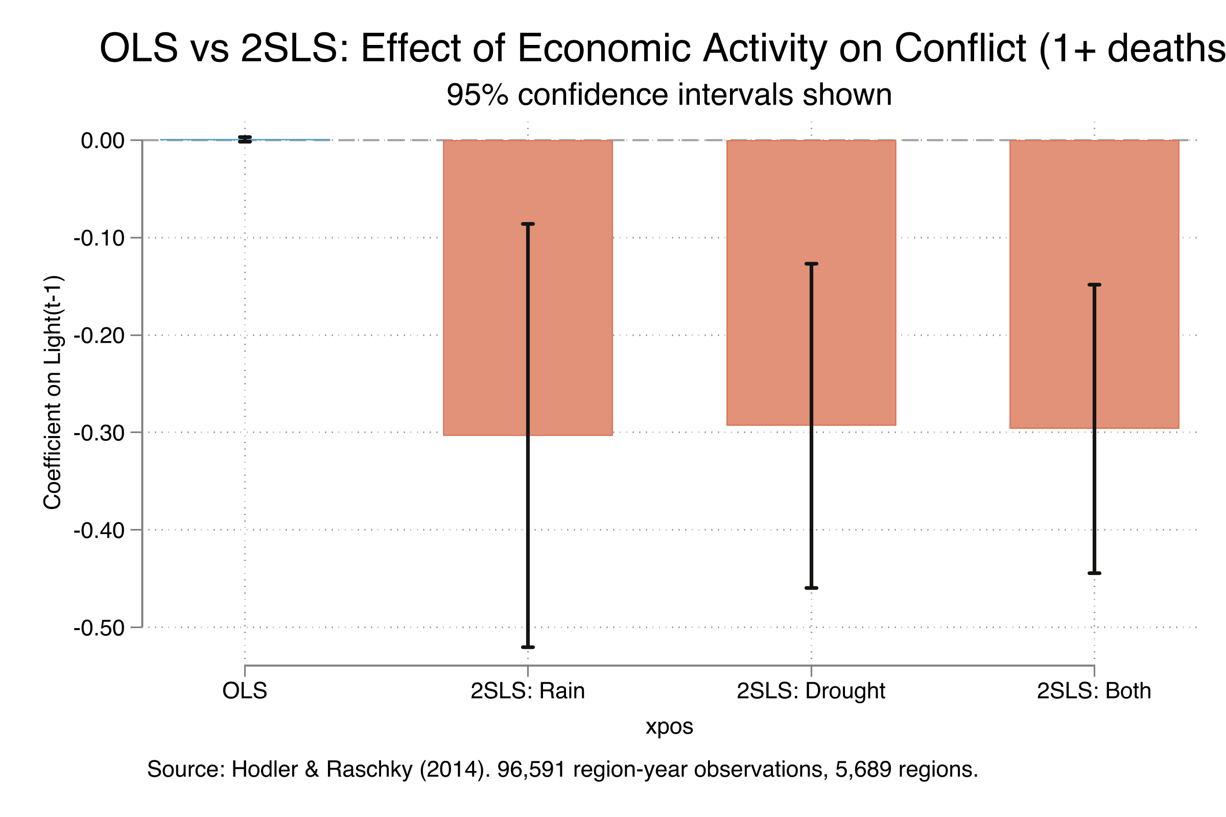
OLS coefficient (steel) is indistinguishable from zero; all three 2SLS estimates (orange) cluster around −0.30 with CIs far from zero.

Spoiler figure — the money chart. Do not explain every bar yet. Just plant that OLS and IV give wildly different answers, and that the IV estimates agree with each other. We earn each one in Act II and return to this picture in Act III.

Where we’re going

• The endogeneity problem: why OLS is the wrong thermometer
• The instrument: lagged weather as exogenous variation in income
• The first stage: do the instruments actually move economic activity?
• 2SLS, the LATE it identifies, and the diagnostics that license it

The Investigation

Act II

Three threats make the OLS slope uninterpretable

• Omitted variables — institutions, geography, ethnic fractionalization drive both income and conflict
• Reverse causality — conflict destroys infrastructure, so conflict lowers lights
• Measurement error — nighttime lights \(\neq\) true GDP, biasing the slope toward zero

The instrumental-variables strategy attacks all three at once — if we can find an exogenous source of variation in economic activity.

This is the endogeneity slide. Economic activity is endogenous in the conflict regression for three distinct reasons, and they need not push the same direction. The OLS slope is a contaminated mix of the causal effect and all three biases.

The lab: 96,591 region-years, 5,689 regions, 53 countries, 1994–2010

• Outcome — binary conflict in a region-year (1+ deaths; also a 25+ deaths version)
• Endogenous regressor — lagged log nighttime light intensity (the income proxy)
• Instruments — lagged log rainfall and lagged drought (Palmer index), two years prior

Region effects, region trends, and year effects are pre-absorbed. SEs clustered on 5,689 regions.

A 5,689-region subnational panel from Hodler & Raschky (2014), taking Miguel, Satyanath & Sergenti’s rainfall-IV idea below the country level. Conflict is rare: only 4.6% of region-years have any conflict death.

The detrended *_dt variables are residuals from region-specific linear trends — equivalent to including those trends in the regression.

Weather two years back drives income, then income drives conflict

The identification rests on a lag chain. Weather at \(t-2\) shifts agricultural output and hence economic activity (lights) at \(t-1\), which then shifts conflict at \(t\).

First stage

\[Light_{i,t-1} = \tilde\delta\, Weather_{i,t-2} + \tilde\alpha_i + \tilde\beta_i t + \tilde\gamma_t + \tilde\varepsilon_{it}\]

Weather predicts income — relevance.

Exclusion

\[Weather_{i,t-2} \not\to Conflict_{i,t}\ \text{(directly)}\]

Weather two years back touches today’s conflict only through income.

The two-year lag is what makes exclusion defensible: weather at t-2 plausibly has no direct line to conflict at t except through the income channel at t-1. This is the standard re-expression of the mermaid DAG from the post (Weather → Light → Conflict, with Weather excluded from Conflict).

The structural equation: \(\delta\) is the causal effect we want

\[Conflict_{it} = \delta\, Light_{i,t-1} + \alpha_i + \beta_i t + \gamma_t + \varepsilon_{it}\]

\(\alpha_i\) are region fixed effects, \(\beta_i t\) region-specific trends, \(\gamma_t\) year effects. The parameter \(\delta\) is the causal effect of economic activity on conflict probability.

This is the second stage. OLS estimates δ inconsistently because Light is endogenous; 2SLS replaces Light with the part of it that weather explains. Same equation, honest estimate.

2SLS identifies a LATE — the effect for weather-driven compliers

Estimand. Not the average effect over all regions. 2SLS recovers the Local Average Treatment Effect (LATE): the effect for the compliers — regions whose economic activity actually responds to weather variation.

Why it can exceed the ATE. Compliers are the more agriculturally exposed regions. Their conflict may be more income-sensitive — but since most African regions are heavily agricultural, the LATE–ATE gap is likely small.

Naming the estimand is mandatory for a causal deck. The IV estimate is local to compliers, not the population ATE. The post’s Section 9 discusses exactly this LATE-vs-ATE distinction.

Two stages: fit lights from weather, then conflict from fitted lights

xtset objectid year
xtivreg2 ucdp_death_dummy_dt ///
    (llnlight01_dt = l2lnrain01_dt l2meanpdsi_dt) Iyear*, ///
    fe robust cluster(objectid) first
* `first` prints the first-stage F; the parentheses mark the endogenous regressor.

xtivreg2 is the panel IV workhorse. The variable in parentheses on the right is the endogenous regressor; the variables after the equals sign are the excluded instruments. fe absorbs the fixed effects, cluster(objectid) gives region-clustered SEs, first requests the first-stage diagnostics. The full do-file is in the post.

Rainfall moves economic activity: a clean positive first stage

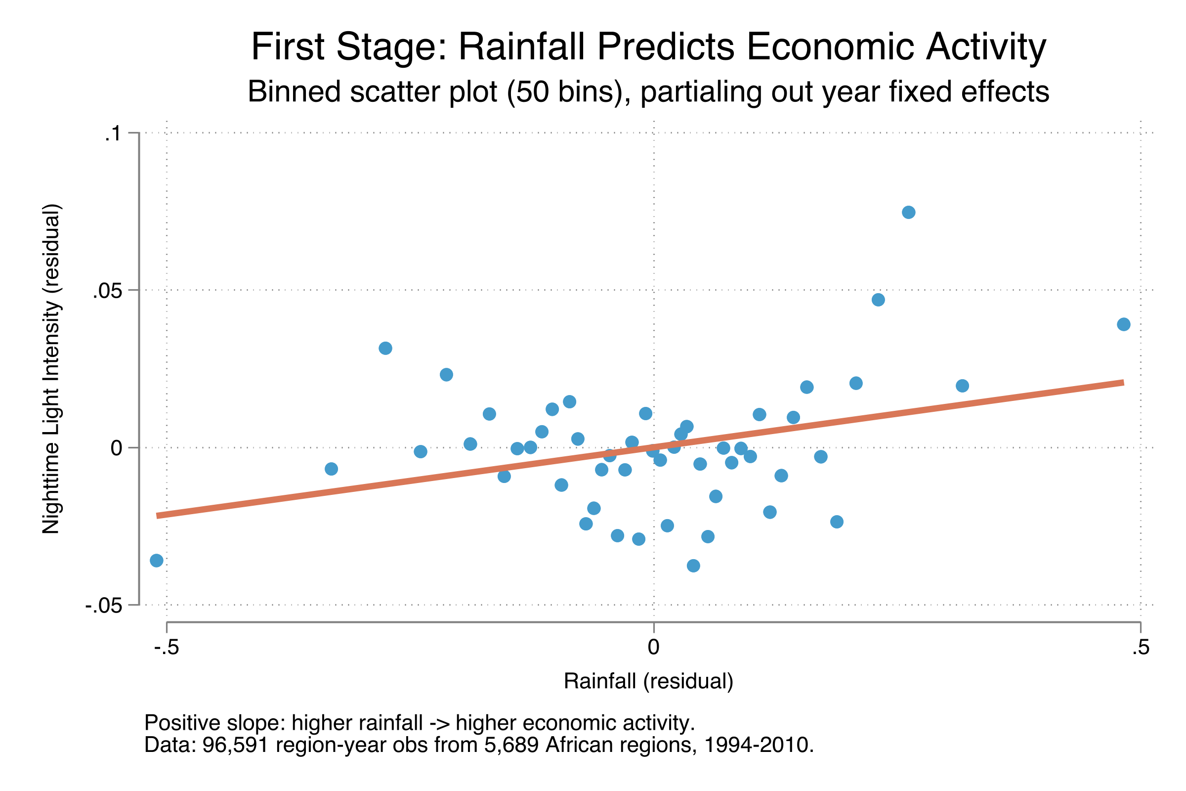
Binned scatter (50 bins) of rainfall residuals vs nightlight residuals, year effects partialled out — a clear upward slope.

First-stage relevance, visualized. Each dot is a bin average after partialing out year fixed effects. More rain → more light next year. First-stage coefficient 0.036 (p < 0.001), F = 24.62.

Drought is the stronger instrument — a tighter first stage

Binned scatter of drought (PDSI) residuals vs nightlight residuals — less drought predicts more economic activity, with a tighter fit than rainfall.

Higher PDSI = less drought → more light. The cloud is tighter than the rainfall plot, foreshadowing the higher first-stage F (40.33 vs 24.62). Drought hits agriculture harder and more directly than rainfall fluctuations.

Both weather instruments move conflict in the reduced form — the IV numerator is real

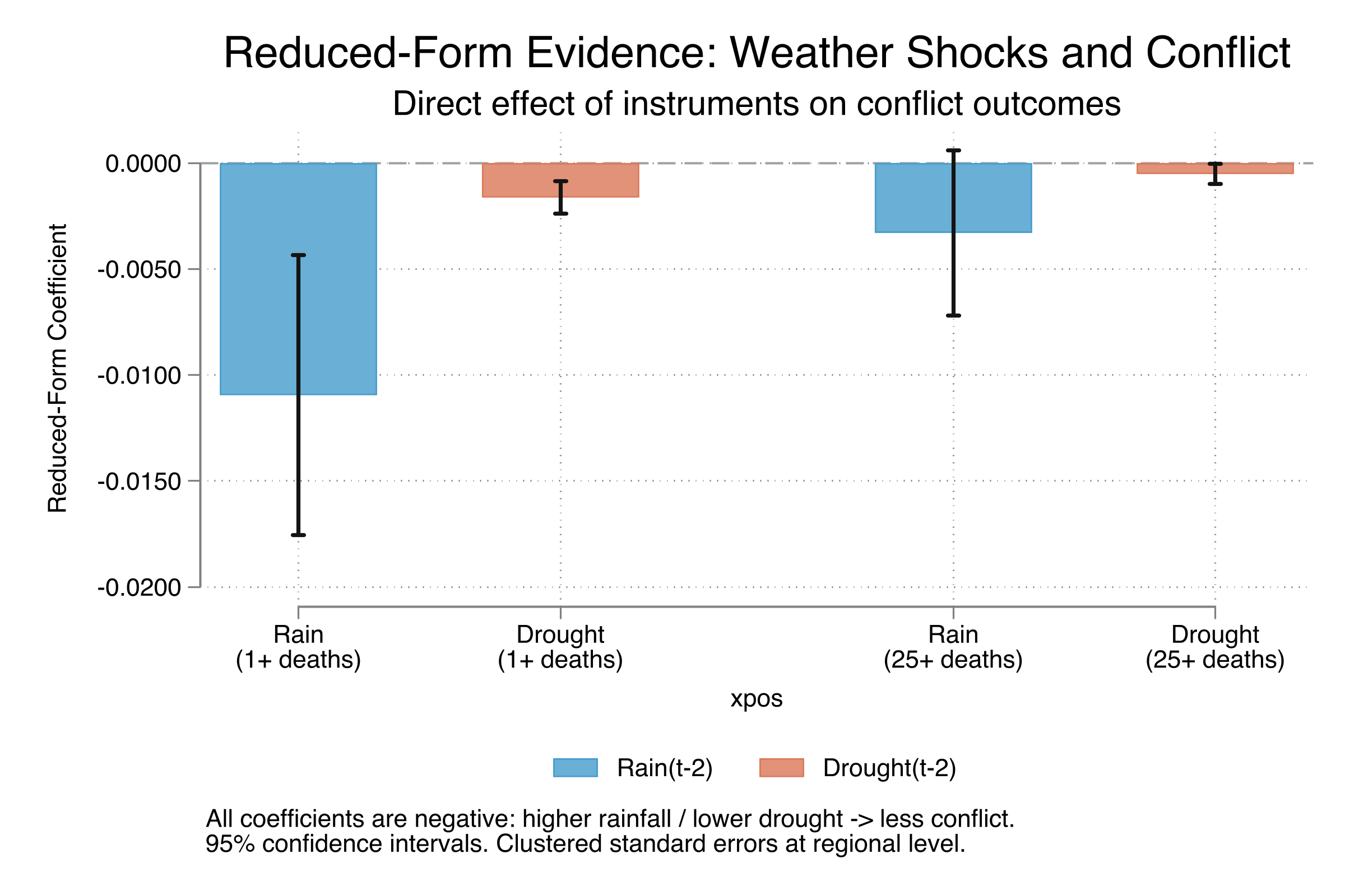
Reduced-form coefficients (weather → conflict): more rain and less drought both predict less future conflict, for both outcomes.

The reduced form is the numerator of the IV ratio. Rainfall → conflict −0.011 (p = 0.001); drought → conflict −0.002 (p < 0.001). Both negative, both in the expected direction. If the instruments had no reduced-form relationship with conflict, there would be nothing for IV to scale up.

Conflict is rare and declining — context for a binary outcome

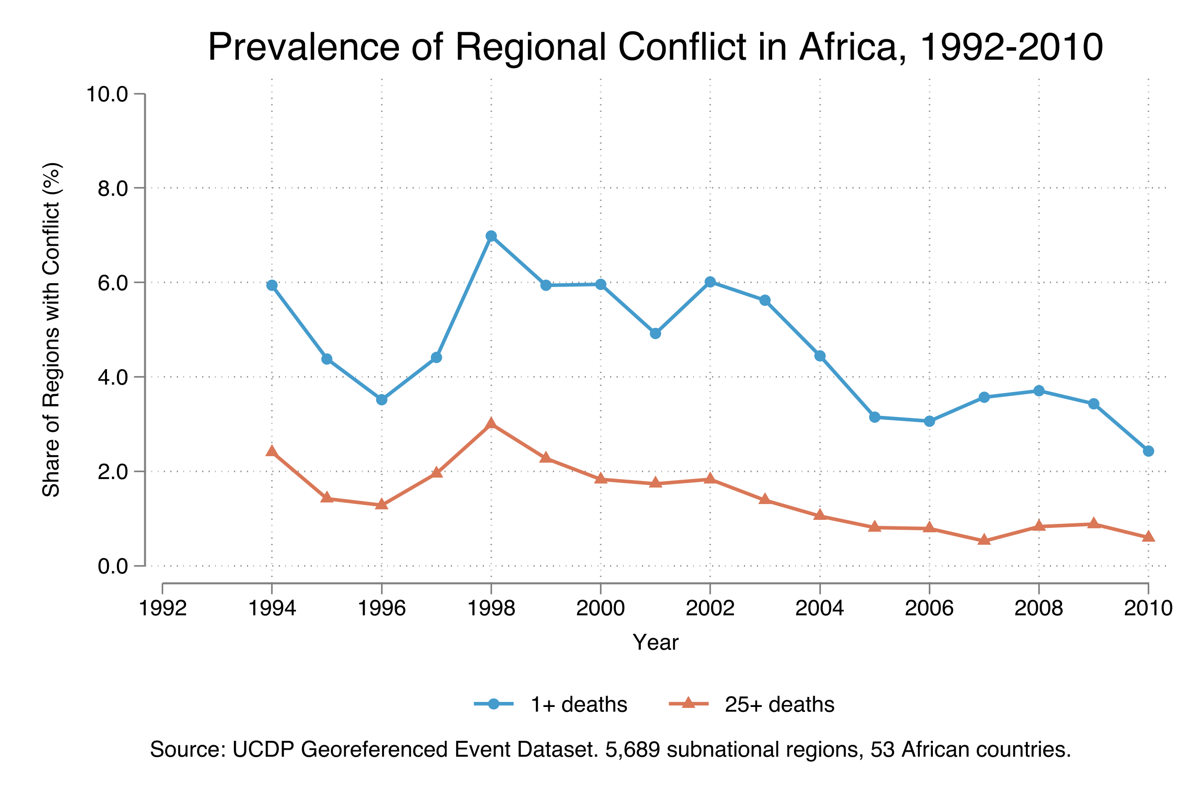
Conflict prevalence by year: any-death conflict (steel) peaks near 7% in 1998 then falls to ~2.5%; severe 25+ death conflict (orange) tracks below at one-third the rate.

Context slide. The outcome is a rare binary event — 4.6% any-death, 1.4% severe. The 1998 peak coincides with the DRC, Ethiopia–Eritrea, and Sierra Leone conflicts. Rarity is why we need strong instruments to pin down the within-region effect.

The Resolution

Act III

Throw out the instruments and OLS reads exactly zero

0.001

OLS coefficient on lights (SE 0.001, p = 0.50) — attenuated to nothing by measurement error

The benchmark that motivates everything. 0.001 is not “no effect” — it is a contaminated thermometer. Classical measurement error in lights shrinks the slope toward zero. Miguel et al. found the same and blamed unreliable African income data.

Instrument the lights and the effect snaps to −0.296

−0.296

2SLS, both instruments (SE 0.076, p < 0.01) — roughly 300-fold the OLS magnitude, opposite sign

The payoff. Once we isolate the weather-driven part of lights, the effect is large, negative, and highly significant. The 300-fold OLS-to-IV gap is the attenuation-bias signature.

Three instrument choices, one answer: −0.293 to −0.303

Instrument	\(\hat\delta_{2SLS}\)	SE	Sig. 1%?
Rain(\(t-2\))	−0.303	0.111	yes
Drought(\(t-2\))	−0.293	0.085	yes
Both	−0.296	0.076	yes

The estimate barely moves across instruments — strong evidence the causal finding is robust, not an artifact of one weather variable.

Robustness as agreement. Three different exogenous shocks, three nearly-identical answers. The “both” column is the most efficient (smallest SE) and is the headline. Contrast with OLS at 0.001 in the same table.

A 10% income drop raises conflict risk by 3 points — a 66% jump

A 10% fall in nighttime lights (\(\approx 0.1\) log units) raises the probability of any-death conflict by about 3 percentage points.

Against a 4.6% baseline, that is a 66% increase in conflict risk — from 4.6% to roughly 7.6% in an average region. For severe (25+ death) conflict the effect is about one-third as large.

Translate the coefficient into something a policymaker feels. −0.296 × 0.1 ≈ −0.030, i.e. a 3-point rise in a 4.6% baseline = +66%. This is the “poverty reduction is conflict prevention” headline.

Strong and valid: every diagnostic clears its threshold

Test	Statistic	Threshold	Verdict
First-stage F (Rain)	24.62	> 16.38	strong
First-stage F (Drought)	40.33	> 16.38	strong
Hansen \(J\) (overid)	\(p = 0.93\)	\(p > 0.10\)	valid

Both instruments clear Stock–Yogo by a wide margin; the overid test says they tell the same story.

Relevance via the first-stage F (both well past Stock-Yogo’s 16.38 for 10% maximal size). Joint validity via Hansen J: with two instruments and one regressor we are overidentified by one, and J = 0.007 (p = 0.93) strongly fails to reject. Strong + consistent = license to believe the IV estimate.

Does IV manufacture causality? No — two assumptions still carry the weight

Objection. Weather instruments don’t prove income causes conflict; you’ve just assumed exclusion.

Response. Correct — identification rests on relevance (testable: F = 24–40) and exclusion (untestable for a single instrument). The two-year lag makes a direct weather→conflict channel implausible, and the Hansen \(J\) shows the two instruments agree. IV disciplines the estimate; it cannot relax the identifying assumptions.

Steelman the critique. The exclusion restriction is fundamentally untestable with exactly one instrument. With two we get the overidentification test as a partial check. The honest claim is conditional: IF weather affects conflict only through income, THEN the effect is −0.30.

When measurement is noisy, the instrument — not OLS — tells the truth.

The single takeaway. OLS read 0.001 because nightlights are a contaminated thermometer; lagged weather is the clean instrument that recovers the real, large, negative effect of economic shocks on civil conflict. Poverty reduction is conflict prevention.