The Synthetic Control Method in Stata

Did California’s Proposition 99 tobacco tax cut smoking?

−19.0ATT · packs per capita / yr

0.974pre-treatment fit (R²)

0.026in-space placebo p-value

Carlos Mendez

Nagoya University (GSID)

June 11, 2026

The Tension

Act I

Smoking was falling everywhere — so did the tax change anything?

In 1988, California voters passed Proposition 99: a 25-cents-per-pack cigarette tax plus funded anti-smoking education, effective January 1989.

But national smoking was already falling. What would California have done without the law?

A simple before-and-after comparison confounds the policy with a trend pushing sales down everywhere. This is the central problem of single-unit policy evaluation. We cannot just compare California before and after 1989, because secular trends — rising health awareness, federal regulation — were already lowering sales nationwide. We need a credible counterfactual: a “California that never passed Prop 99.”

A raw comparison hints at an effect — but the comparator is crude

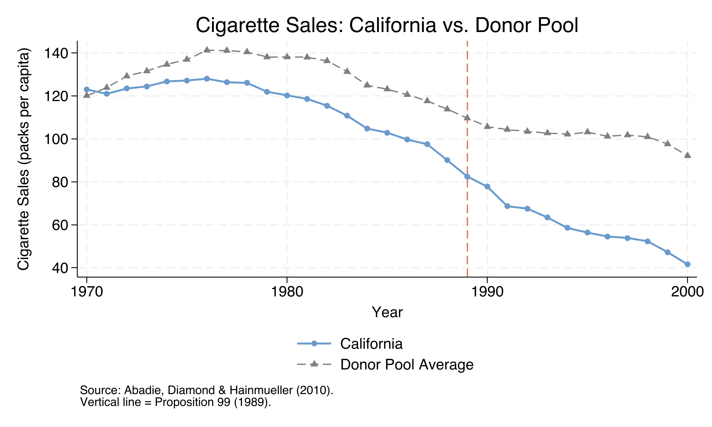
Cigarette sales per capita: California (solid blue) vs. the unweighted average of 38 control states (dashed grey), 1970–2000. Orange line marks Prop 99 (1989).

Before 1989 California broadly tracks the donor-pool average, then drops sharply. But the unweighted average gives equal weight to Kentucky (213 packs) and Utah (64 packs) — states with nothing like California’s smoking profile. We need an optimal weighted comparator. That is the synthetic control.

Where we’re going

• The lab: a 39-state, 31-year panel and the ATT estimand
• Build “synthetic California” with synth2 — a weighted blend of donor states
• Three inference tools: in-space placebo, in-time placebo, leave-one-out
• The lesson: a transparent counterfactual beats parallel-trends faith

The Investigation

Act II

The lab: 39 states × 31 years, one treated unit, the ATT

• Outcome — cigsale, per-capita cigarette sales (packs)
• Treatment — Prop 99, California only, from 1989
• Predictors — log income, share aged 15–24, retail price, beer, plus cigsale in 1975/1980/1988

Strongly balanced: 1,209 observations, 19 pre-treatment years and 12 post-treatment years. The estimand is the ATT — the effect on California, the one treated unit — not the ATE.

With a single treated unit and aggregate data, difference-in-differences’ parallel-trends assumption is hard to test. SCM instead builds an explicit counterfactual and lets you see the match quality in the pre-treatment period. California is state == 3 in the data.

SCM builds a counterfactual by matching pre-treatment predictors

\[\min_{W} \sum_{m=1}^{M} v_m \left( X_{1m} - \sum_{j=2}^{J+1} w_j X_{jm} \right)^2\]

Pick donor weights \(w_j \ge 0\) that sum to one and match California’s predictors \(X_{1m}\).

The weights \(v_m\) set how much each covariate matters.

The synthetic control is a convex combination of real states — no extrapolation beyond the donor pool.

This is a nested optimization. The outer problem picks the V-weights (predictor importance); the inner problem picks the W-weights (donor shares) that minimize the weighted predictor distance. The non-negativity and sum-to-one constraints are what keep the synthetic interpretable and guard against overfitting.

The treatment effect is the gap between actual and synthetic California

\[\hat{\tau}_t = Y_{1t} - \sum_{j=2}^{J+1} w_j^* Y_{jt}\]

The effect in year \(t\) is California’s actual sales minus the synthetic’s prediction. A negative \(\hat{\tau}_t\) means Prop 99 lowered sales.

Identification rests on good pre-treatment fit, no interference, and no anticipation — assumptions you can largely inspect, not just assume.

The ATT is the mean of these yearly gaps over 1989–2000. Unlike DiD, you do not need parallel trends as an article of faith. If the synthetic tracks the real unit closely before treatment, the post-treatment divergence is credibly the effect. The three assumptions: Prop 99 did not change other states’ sales (no interference), donors did not pass similar laws pre-1989 (no anticipation), and the synthetic reproduces the pre-1989 path (good fit).

One synth2 call fits the baseline synthetic control

synth2 cigsale lnincome age15to24 retprice beer ///
    cigsale(1988) cigsale(1980) cigsale(1975), ///
    trunit(3) trperiod(1989) xperiod(1980(1)1988) nested allopt

trunit(3) = California · trperiod(1989) = treatment year · nested = outer V / inner W · allopt = multiple starts to dodge local optima.

Seven predictors: four economic/demographic variables averaged over 1980–1988, plus cigarette sales at three pre-treatment anchor years (1975, 1980, 1988). The nested allopt combination is the gold-standard specification — slower, but it avoids spurious local optima in the V-weight search.

Synthetic California reproduces 97.4% of the pre-1989 path

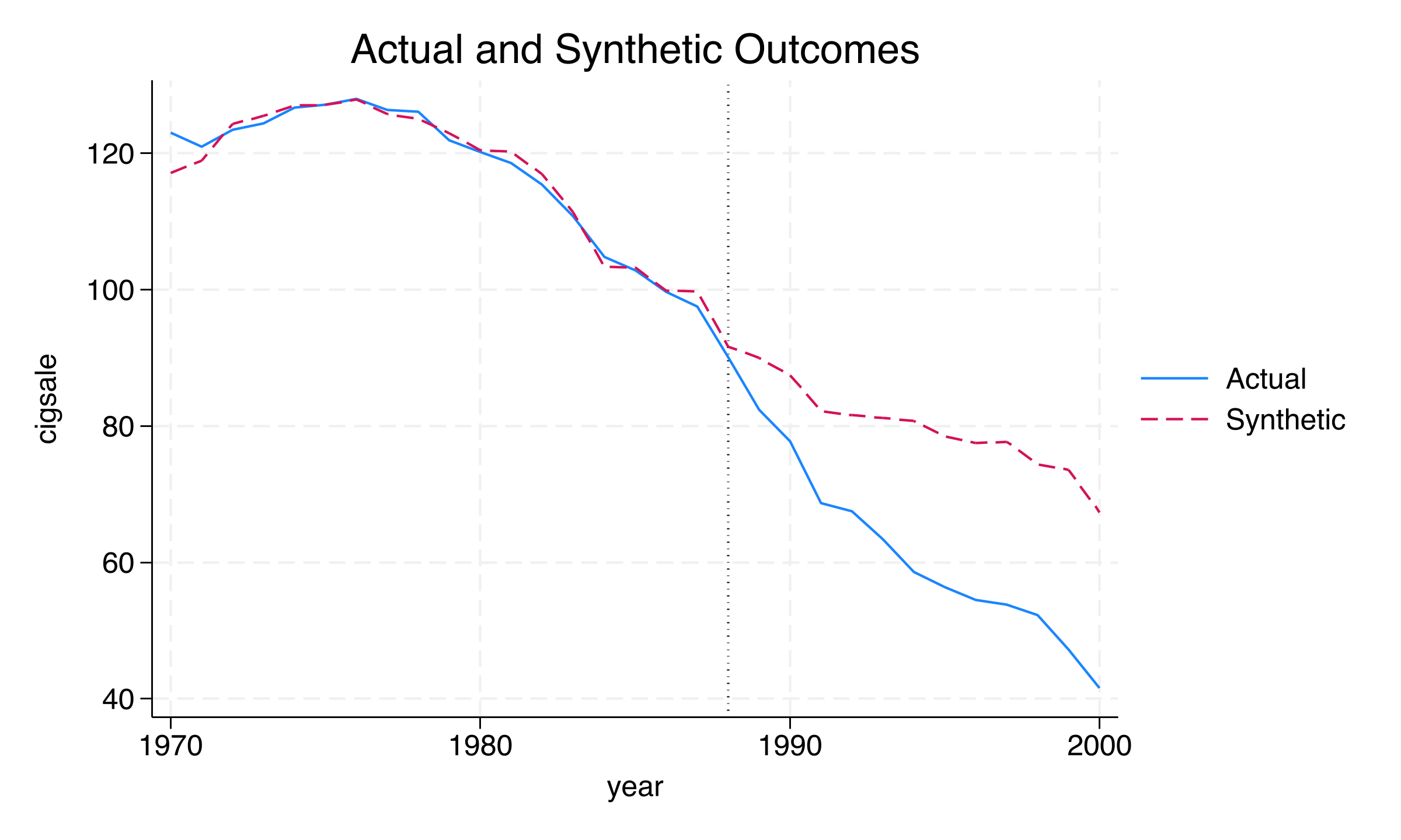
California actual vs. synthetic California, 1970–2000: near-indistinguishable before 1989, then a widening gap.

R-squared = 0.974, RMSE = 1.76 packs over 19 pre-treatment years — an excellent fit. The two lines are visually inseparable from 1970 to 1988. Because the match is this good, we can trust that the post-1989 divergence reflects the policy, not pre-existing differences.

Two predictors carry the match: age 15–24 and 1975 sales

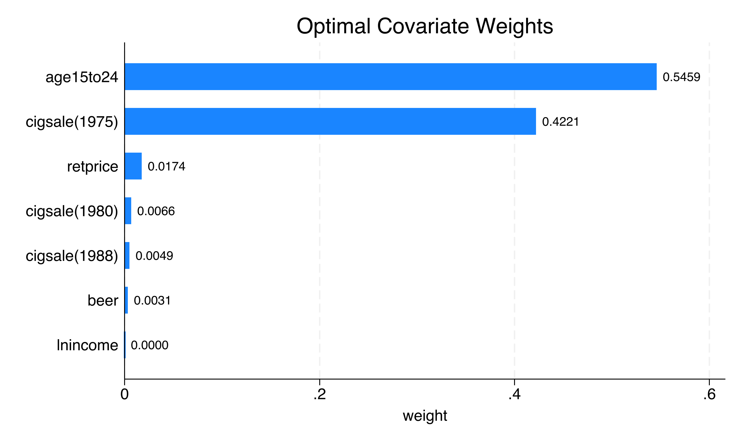
Predictor (V-matrix) weights: how much each covariate drives the SCM optimization.

The dominant V-weights are age 15–24 (0.546) and cigsale(1975) (0.422). Log income gets essentially zero weight — it does little to distinguish California from its synthetic twin. All seven predictor biases are below 2.2%, with five below 0.3%; the simple average control, by contrast, is off by 26% on 1988 sales.

Synthetic California is just five states — one-third Utah

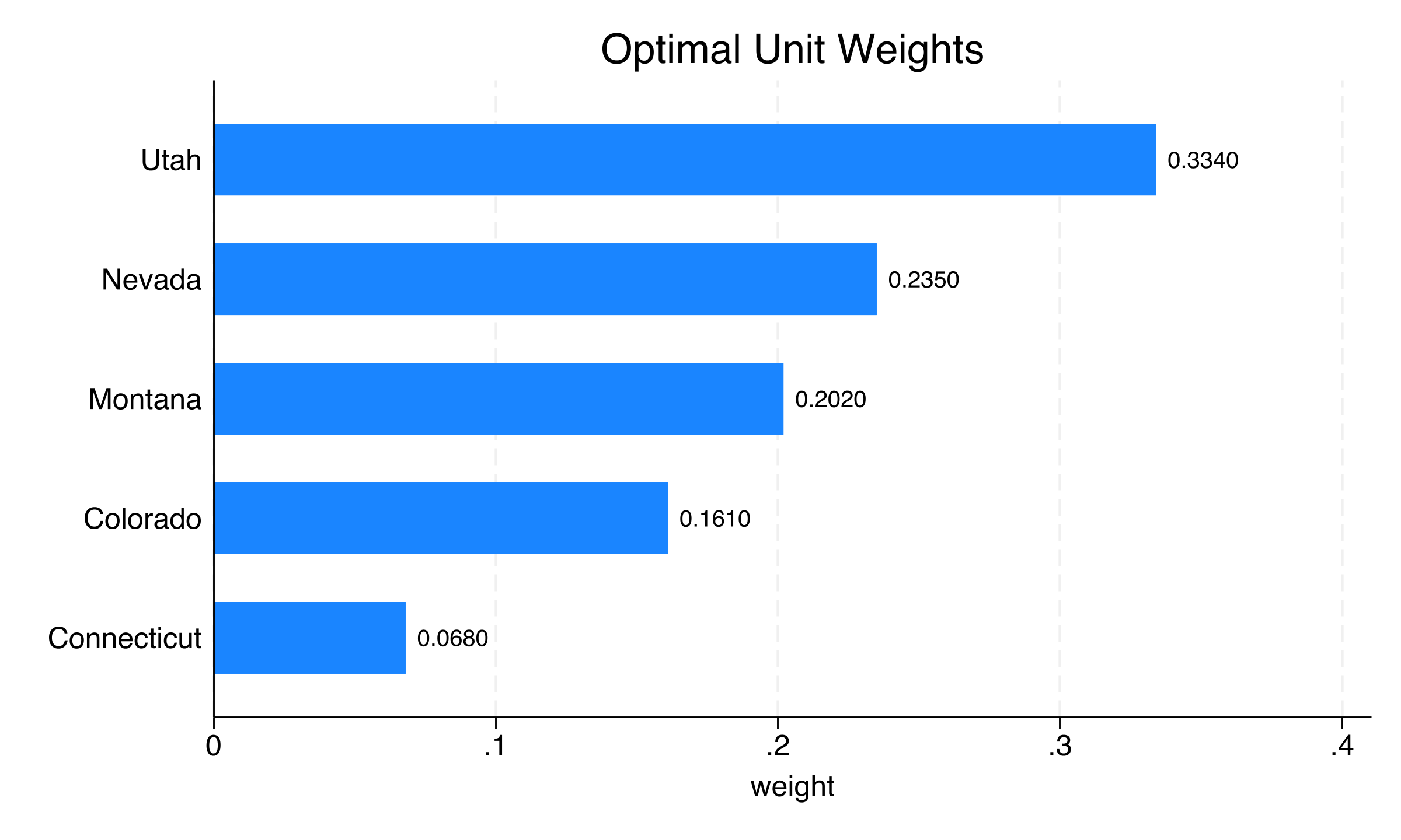
Donor weights: the five states that compose synthetic California (33 others get exactly zero).

Utah 33.4%, Nevada 23.5%, Montana 20.2%, Colorado 16.1%, Connecticut 6.8%. SCM is inherently sparse — it picks states by trajectory similarity, not geographic proximity. That Utah carries a third of the weight is exactly why we will run leave-one-out later.

By 2000, real California sold 38% fewer packs than its synthetic twin

−19.0

average ATT, packs per capita / yr (1989–2000); −7.6 in 1989 deepening to −26.4 by 1999

The effect compounds. By 2000 California’s actual sales (41.6 packs) sit 25.8 packs below the synthetic (67.4) — a 38% reduction. For ~34 million residents that is roughly 900 million fewer packs sold per year. The growing gap is consistent with cumulative behavioral change and shifting social norms.

The gap deepens steadily through the 1990s

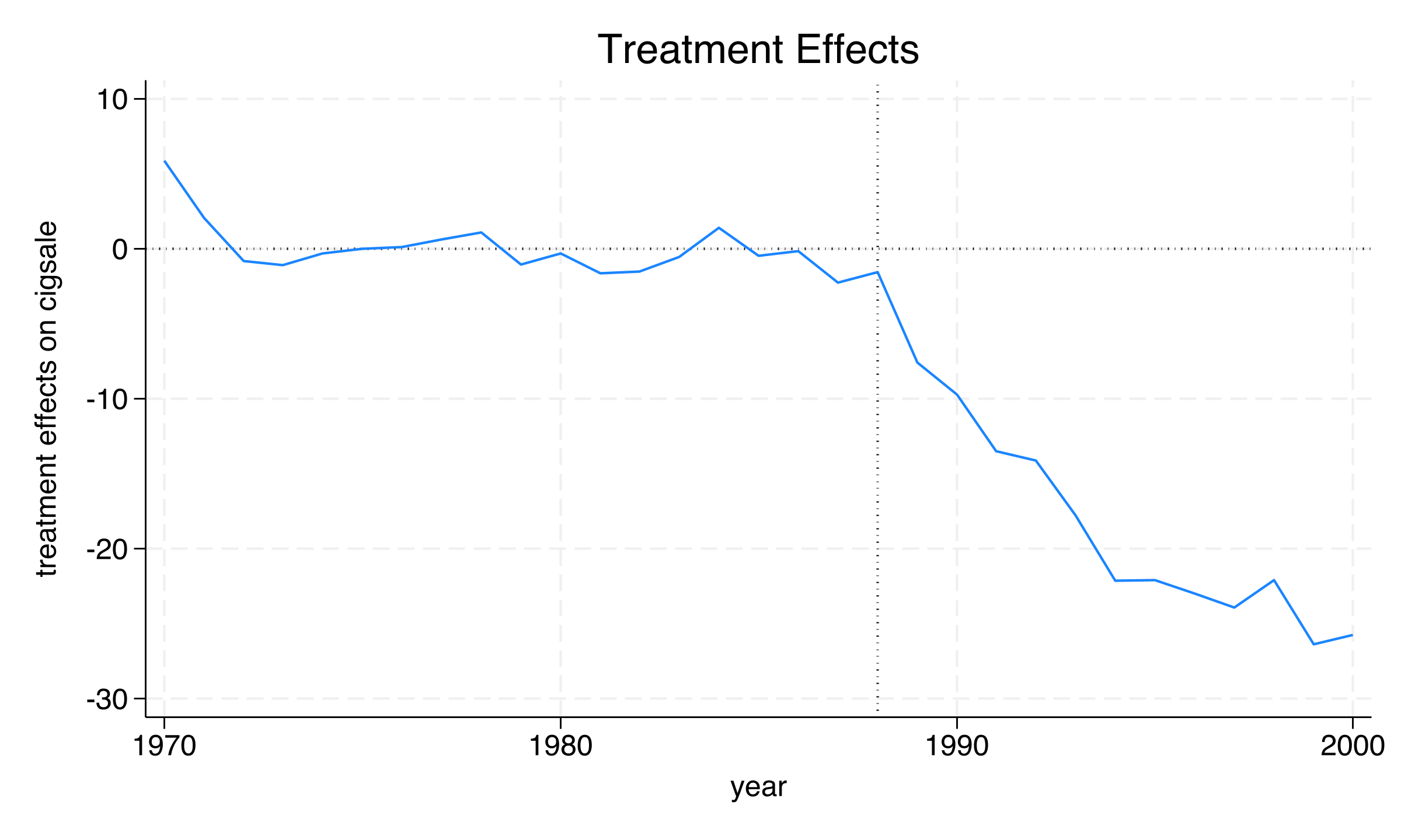
Treatment effect (actual minus synthetic California) over time; the negative gap widens after 1989.

Effect starts at −7.6 packs (1989), reaches −26.4 by 1999, plateaus near −25 to −26 in 1999–2000. But is this real, or could a never-treated state show a gap this large by chance? Act III stress-tests it three ways.

The Resolution

Act III

California’s signal-to-noise ratio is the most extreme of all 39 states

State	Pre MSPE	Post/Pre MSPE
California	3.17	123.5
Georgia	1.46	80.0
Virginia	2.78	79.0
Missouri	1.20	70.9

The post/pre MSPE ratio asks: how much worse does fit get after 1989 than before? California’s is highest by far.

A genuine effect should blow up the post-treatment prediction error relative to a small pre-treatment error. California’s ratio of 123.5 dwarfs the runners-up. This is the conservative inference statistic — it rewards both a large gap AND a tight pre-treatment fit.

Run the placebo on every state — California is the lone outlier

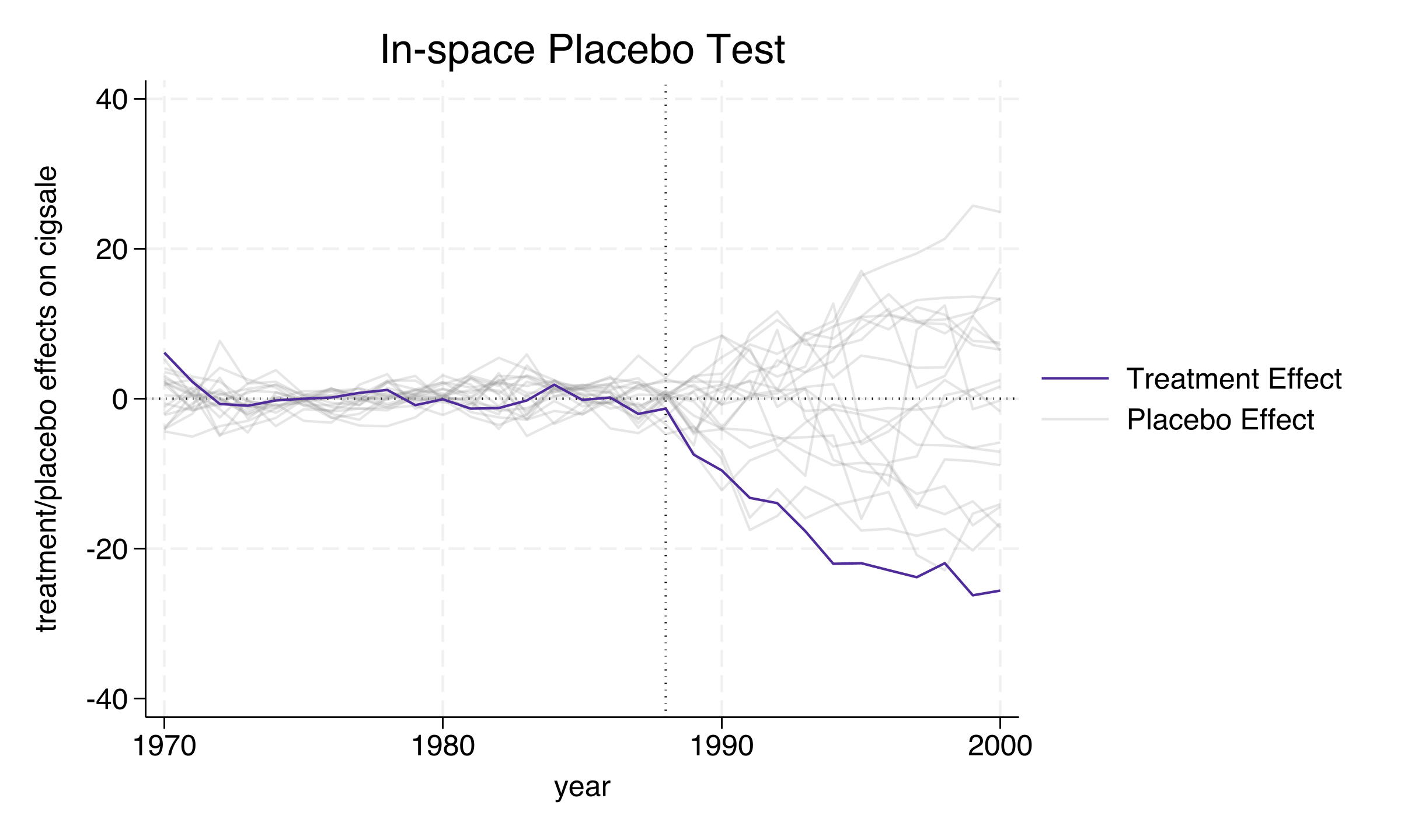
Treatment effects for all states: California (bold) plunges away from the tight grey band of placebo gaps near zero.

The in-space placebo applies the same SCM to each control state, pretending each was treated in 1989. This is a permutation test: if we randomly assigned “treatment” to any state, how often would we see a gap as large as California’s? Almost never — California’s trajectory is a dramatic visual outlier.

Across all 39 states, a gap this large appears 2.6% of the time

0.026

in-space placebo p-value, all controls (1/39); p = 0.05 after the cut(2) fit filter (1/20)

Using all states, p = 0.026. After the cut(2) filter removes 19 states whose pre-treatment MSPE exceeds twice California’s, 20 states remain and p = 1/20 = 0.05 — right at the threshold, a mechanical consequence of having few comparison units. Report both: the unfiltered p is more conservative; the filtered one is fairer.

Significance holds in most post-treatment years

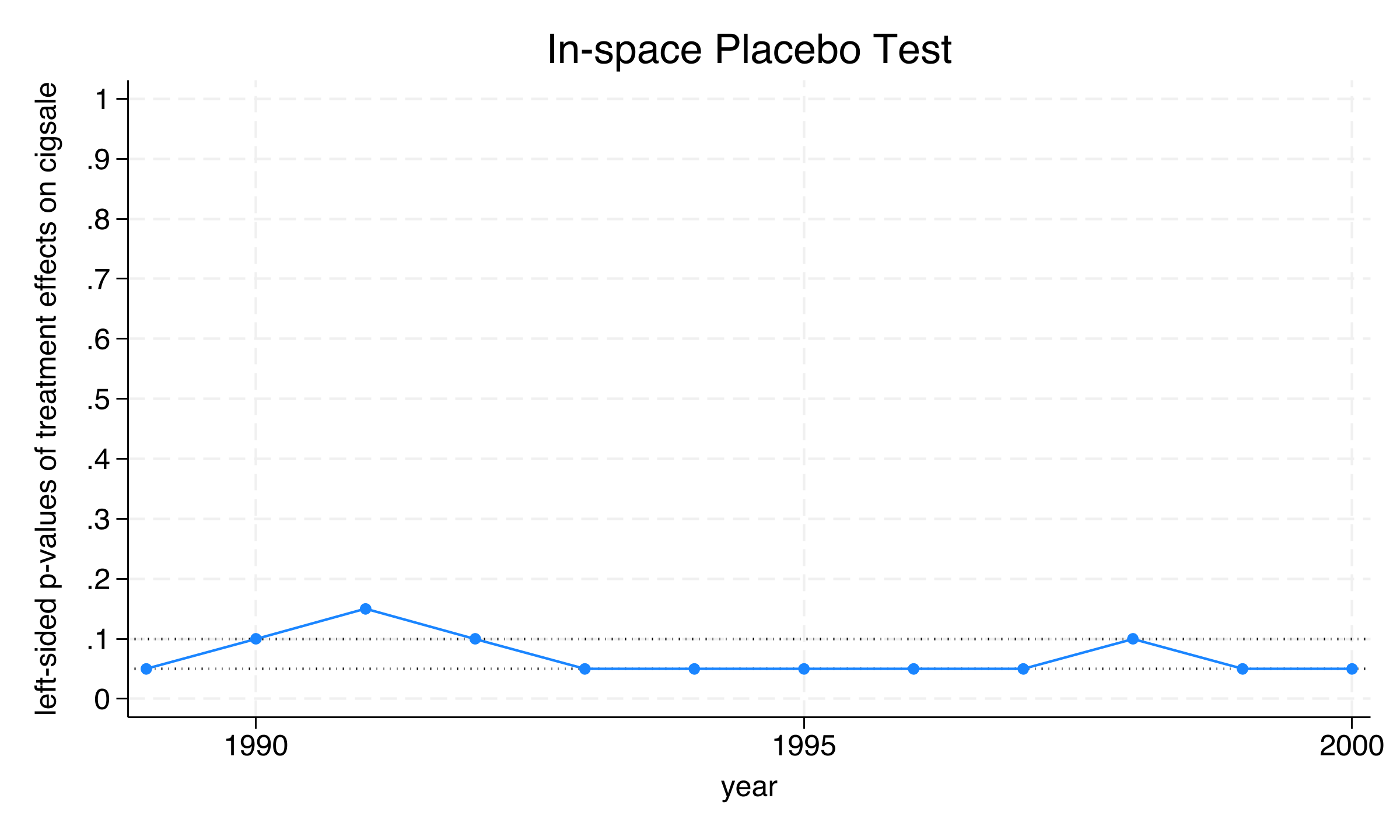
Left-sided Fisher exact p-values over time (left-sided, because the effect is negative): p = 0.05 in most years.

Left-sided p-values are the right choice for a negative effect. They equal 0.05 in 8 of 12 post-treatment years; the weaker years (1990–1992 and 1998, p = 0.10–0.15) are exactly when the effect was still small in magnitude. From 1993 on, California is the most extreme state in most years.

A fake 1985 treatment produces no comparable gap

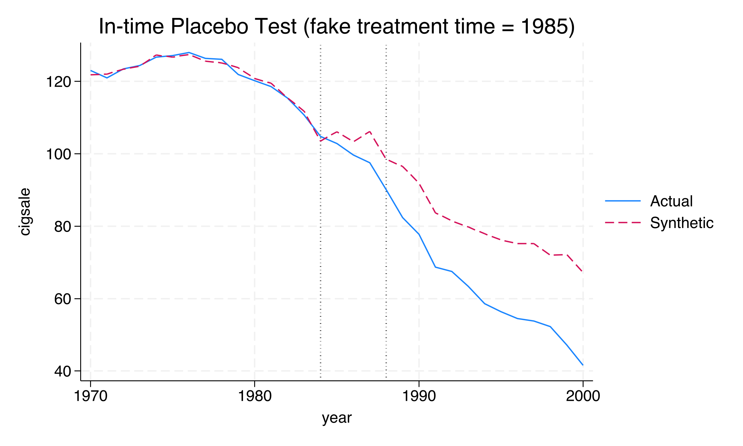
In-time placebo: California actual vs. synthetic with a fake treatment at 1985. Lines stay close through 1988, then split after the real 1989 policy.

If the design were spurious, a fake earlier treatment date would manufacture an effect. Instead, fake-period effects (1985–1988) are only −3.3 to −8.7 packs — versus −14.1 to −25.6 after 1989. The sharp discontinuity lands precisely at 1989. The non-zero fake effects reflect the shorter training window (R² drops to 0.953), not a real pre-trend.

The effect snaps on at the real date, not the fake one

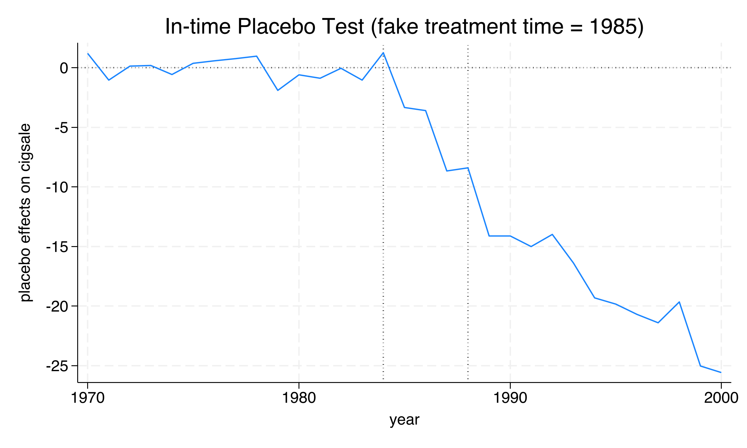
In-time placebo effect: small gaps during the fake 1985–1988 window, large gaps after the real 1989 treatment.

Fake-period effects average about −6.0 packs; real-period effects roughly double at 1989 (−8.4 in 1988 to −14.1 in 1989) and keep deepening. The model does not detect a large effect where none should exist — strong internal-validity evidence.

No single donor drives the result — leave-one-out stays negative

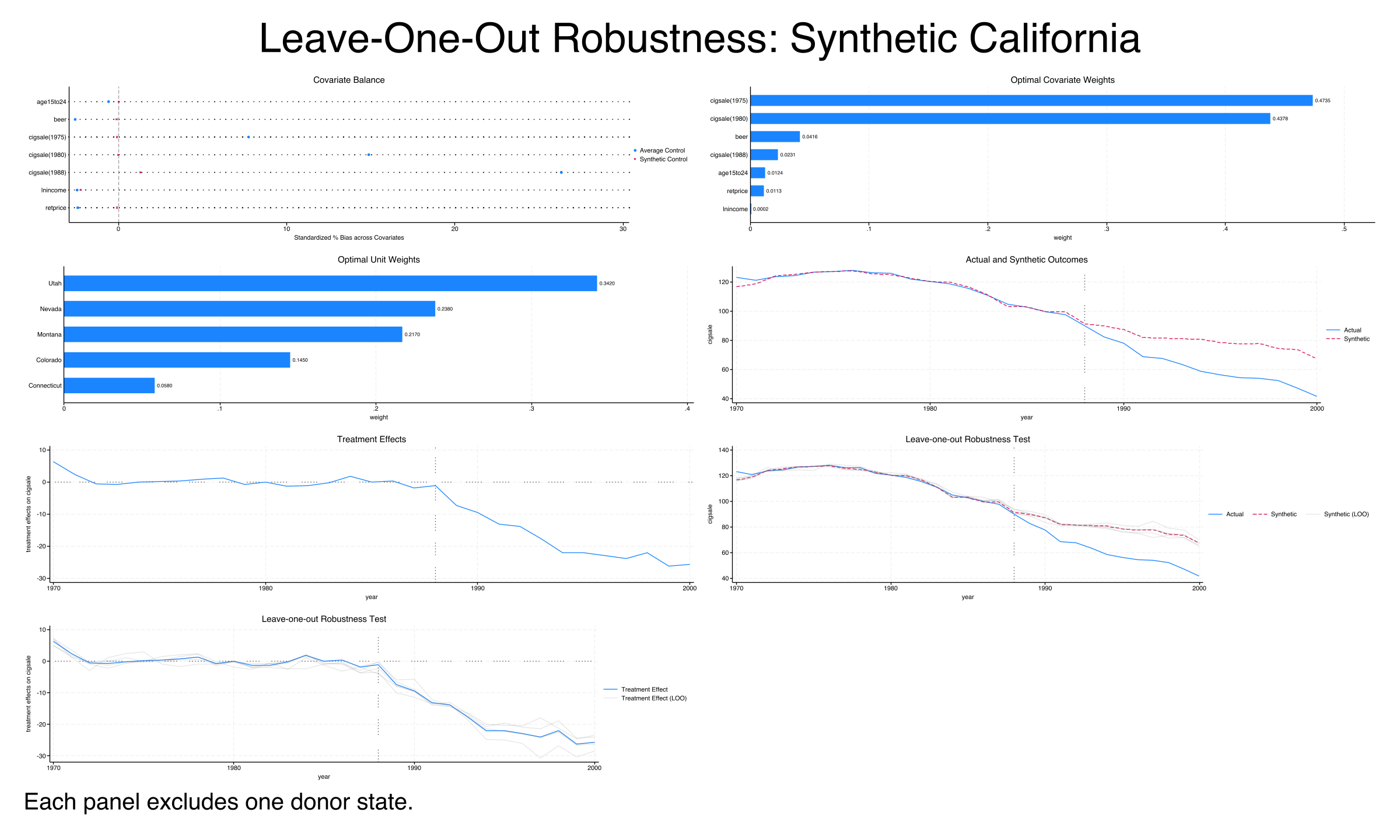
Leave-one-out: synthetic California’s prediction stays similar whichever weighted donor state is dropped.

Drop each of the five weighted donors in turn. For 2000 the LOO range is [−28.4, −23.5] around a baseline of −25.6 — a 4.9-pack spread, ~19% of the estimate. No iteration approaches zero, even when Utah (a third of the weight) is removed. The leave-one-out estimates stay close to the baseline ATT of −19.0 packs.

Does choosing controls by fit make this causal? Not by itself

Objection. A flexible, data-driven counterfactual still can’t manufacture identification.

Response. Correct. The ATT is credible only under no interference, no anticipation, and good pre-treatment fit — SCM makes the last one visible and disciplines the comparator, but it cannot rule out cross-border shopping or an idiosyncratic donor (e.g. Utah’s distinct smoking norms). It also gives no standard errors; inference rides entirely on the placebos.

Steelman the critique. SCM’s value is transparency, not a free identification lunch. The five-state synthetic is sensitive to the predictor set (ATT moves from −19.0 to −17.7 in the in-time spec), and the donor pool deliberately excludes states with their own tobacco programs. Recent conformal-inference methods offer more formal confidence intervals.

Let the pre-treatment fit — not a parallel-trends assumption — earn your counterfactual.

The single takeaway. With one treated unit, a transparent weighted counterfactual you can validate before treatment is more honest than an untestable parallel-trends story. For California, three independent checks — placebo in space, placebo in time, and leave-one-out — all point the same way: Prop 99 cut smoking, by about 19 packs per capita per year.