Spatial Panel Regression in Stata: Cigarette Demand Across US States
1. Overview
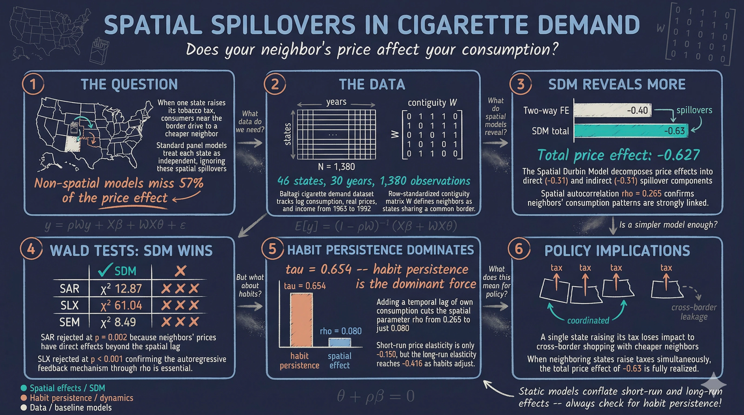
Cigarette taxation is a state-level policy instrument, but consumption in one state does not exist in isolation. When a state raises its tobacco tax, consumers near state borders may simply drive across to buy cheaper cigarettes in a neighboring state. This cross-border shopping effect means that a state’s cigarette consumption depends not only on its own prices and income but also on the prices and income of its neighbors. Standard panel data models — pooled OLS, fixed effects, and two-way fixed effects — cannot capture these spatial spillovers because they treat each state as an independent observation.
This tutorial introduces spatial panel regression as a framework for modeling geographic interdependence in panel data. We use the classic Baltagi cigarette demand dataset, which tracks per-capita cigarette consumption, real prices, and real per-capita income across 46 US states from 1963 to 1992. Starting from non-spatial panel models as a baseline, we progressively build toward the Spatial Durbin Model (SDM) — a flexible specification that includes both the spatial lag of the dependent variable and spatial lags of the explanatory variables. We then use Wald tests to determine whether simpler spatial models (SAR, SLX, or SEM) are adequate, and finally extend the framework to dynamic spatial panels that account for habit persistence in cigarette consumption.
All estimation is performed using the xsmle package in Stata, which implements maximum likelihood estimation for a family of spatial panel models with fixed effects. The spatial weight matrix is a binary contiguity matrix that defines two states as neighbors if they share a common border, row-standardized so that the spatial lag of a variable equals the average value among a state’s neighbors.
Learning objectives
- Estimate non-spatial panel models (pooled OLS, region FE, time FE, two-way FE) and compare their price and income elasticities
- Construct and load a row-standardized spatial weight matrix for panel data in Stata
- Estimate the Spatial Durbin Model (SDM) with two-way fixed effects using the
xsmlepackage - Apply the Lee and Yu bias correction for spatial panels with moderate time dimensions
- Use Wald tests to evaluate whether the SDM simplifies to SAR, SLX, or SEM
- Estimate dynamic spatial panel models with temporal and spatiotemporal lags to capture habit persistence
2. The modeling pipeline
The tutorial follows a progressive approach — each stage builds on the previous one by relaxing assumptions and adding complexity. The diagram below summarizes the path from data preparation through the final dynamic spatial models.
graph LR
    A["<b>Data & W</b><br/><i>Section 3</i><br/>Panel setup<br/>Weight matrix"]
    B["<b>Non-Spatial</b><br/><i>Section 4</i><br/>OLS, FE,<br/>Two-way FE"]
    C["<b>SDM</b><br/><i>Section 6</i><br/>Spatial Durbin<br/>+ Lee-Yu"]
    D["<b>Wald Tests</b><br/><i>Section 7</i><br/>SAR? SLX?<br/>SEM?"]
    E["<b>Dynamic</b><br/><i>Section 8</i><br/>Temporal &<br/>spatial lags"]

    A --> B
    B --> C
    C --> D
    D --> E

    style A fill:#6a9bcc,stroke:#141413,color:#fff
    style B fill:#d97757,stroke:#141413,color:#fff
    style C fill:#00d4c8,stroke:#141413,color:#141413
    style D fill:#141413,stroke:#d97757,color:#fff
    style E fill:#6a9bcc,stroke:#141413,color:#fff
We first establish non-spatial benchmarks to understand the baseline price and income elasticities. Then we introduce the Spatial Durbin Model to capture spillovers, apply Wald tests to check whether a simpler spatial specification suffices, and finally add dynamic components to account for the habit-forming nature of cigarette consumption.
3. Setup and data loading
Before running any spatial models, we need three Stata packages: spmat for spatial weight matrix management, xsmle for spatial panel estimation, and spwmatrix for weight matrix conversion. If you have not installed them, uncomment the net install lines below.
clear all
macro drop _all
set more off
version 12

* Install packages (uncomment if needed)
*net install st0292, from(http://www.stata-journal.com/software/sj13-2)
*net install xsmle, from(http://fmwww.bc.edu/RePEc/bocode/x)
*net install spwmatrix, from(http://fmwww.bc.edu/RePEc/bocode/s)
3.1 Spatial weight matrix
The spatial weight matrix W defines the neighborhood structure among the 46 US states. We use a binary contiguity matrix where two states are neighbors if they share a common border. The matrix is stored in a .dta file and converted to an spmat object with row-standardization — meaning that each row sums to one, so the spatial lag of a variable equals the weighted average among a state’s neighbors.
* Load binary contiguity W matrix and convert to row-standardized spmat object
use "https://github.com/quarcs-lab/data-open/raw/master/cigar/Wct_bin.dta", replace
spmat dta Wst m1-m46, norm(row) replace
The spmat dta command reads columns m1 through m46 from the loaded dataset and stores them as a spatial weight matrix object named Wst. The norm(row) option applies row-standardization, and replace overwrites any existing matrix with the same name.
3.2 Panel data setup
The Baltagi cigarette demand dataset contains three variables measured across 46 US states and 30 years (1963–1992): log per-capita cigarette consumption (logc), log real cigarette price (logp), and log real per-capita disposable income (logy).
* Load panel data
use "https://github.com/quarcs-lab/data-open/raw/master/cigar/baltagi_cigar.dta", clear
sort year state
xtset state year
Panel variable: state (strongly balanced)
 Time variable: year, 1963 to 1992
         Delta: 1 unit
The panel is strongly balanced — all 46 states are observed in all 30 years, yielding 1,380 total observations. This balanced structure simplifies estimation and avoids the complications of missing data.
3.3 Panel summary statistics
The xtsum command decomposes each variable’s variation into between-state and within-state components — a key diagnostic for understanding what panel models can and cannot identify.
xtsum
Variable         |      Mean   Std. dev.       Min        Max |    Observations
-----------------+--------------------------------------------+----------------
logc     overall |  4.625563   .2538233   3.736352   5.399758 |     N =    1380
         between |              .225498   4.057739    5.19628 |     n =      46
         within  |             .1254968   4.110718   5.070093 |     T =      30
                 |                                            |
logp     overall |  3.648067   .3364439   2.579455   4.588055 |     N =    1380
         between |             .1927783    3.22723   4.021831 |     n =      46
         within  |             .2798008   2.780289   4.372397 |     T =      30
                 |                                            |
logy     overall |  1.615786    .248717   .8676362   2.253795 |     N =    1380
         between |             .1363281   1.294913   2.063736 |     n =      46
         within  |             .2098697   1.035539   2.106283 |     T =      30
Variables
| Variable | Description | Mean | Std. Dev. |
|---|---|---|---|
logc |
Log per-capita cigarette consumption (packs) | 4.626 | 0.254 |
logp |
Log real price per pack (cents) | 3.648 | 0.336 |
logy |
Log real per-capita disposable income | 1.616 | 0.249 |
Mean log consumption is 4.63, corresponding to roughly 102 packs per capita per year. The between-state standard deviation of logc (0.225) is larger than the within-state standard deviation (0.125), indicating that cross-state differences in consumption levels are more pronounced than changes within a single state over time. For logp, the pattern reverses — within-state variation (0.280) exceeds between-state variation (0.193), reflecting the fact that real prices changed substantially over this 30-year period due to tax policy changes and inflation. This decomposition foreshadows why fixed effects models, which exploit within-state variation, may produce different elasticity estimates than pooled models.
4. Non-spatial panel models
Before introducing spatial dependence, we estimate four standard panel specifications to establish baseline price and income elasticities. Each model relaxes a different assumption about unobserved heterogeneity, and comparing their estimates reveals how sensitive the results are to the treatment of state-level and time-level confounders.
4.1 Pooled OLS
Pooled OLS treats all 1,380 observations as independent, ignoring the panel structure entirely. It provides a naive benchmark.
reg logc logp logy
estimates store pool
      Source |       SS           df       MS      Number of obs   =     1,380
-------------+----------------------------------   F(2, 1377)      =    199.28
       Model |  21.564818         2  10.7824090   Prob > F        =    0.0000
    Residual |  74.518523     1,377  .054116576   R-squared       =    0.2244
-------------+----------------------------------   Adj R-squared   =    0.2233
       Total |  96.083341     1,379  .069676098   Root MSE        =    .23284

------------------------------------------------------------------------------
        logc | Coefficient  Std. err.      t    P>|t|     [95% conf. interval]
-------------+----------------------------------------------------------------
        logp |  -.3857227   .0309752   -12.45   0.000    -.4464987   -.3249467
        logy |   .3724439   .0264568    14.08   0.000     .3205328    .4243551
       _cons |   4.396312   .0531992    82.64   0.000     4.291951    4.500674
------------------------------------------------------------------------------
Pooled OLS estimates a price elasticity of -0.386 and an income elasticity of 0.372, both statistically significant at the 1% level. However, the R-squared is only 0.224, and more importantly, this model assumes no systematic differences across states — an untenable assumption given the large between-state variation we observed in the summary statistics.
4.2 Region fixed effects
Region (state) fixed effects control for all time-invariant state characteristics — geographic location, cultural attitudes toward smoking, historical tobacco production, and any other state-specific factor that does not change over the sample period.
xtreg logc logp logy, fe
estimates store rfe
Fixed-effects (within) regression               Number of obs     =      1,380
Group variable: state                            Number of groups  =         46

R-squared:                                       Obs per group:
     Within  = 0.4059                                         min =         30
     Between = 0.0681                                         avg =       30.0
     Overall = 0.1050                                         max =         30

                                                 F(2,1332)         =     455.52
corr(u_i, Xb) = -0.8072                         Prob > F          =     0.0000

------------------------------------------------------------------------------
        logc | Coefficient  Std. err.      t    P>|t|     [95% conf. interval]
-------------+----------------------------------------------------------------
        logp |  -.2307217   .0276419    -8.35   0.000    -.2849426   -.1765008
        logy |  -.0145419   .0389849    -0.37   0.709    -.0910300    .0619462
       _cons |   4.619736   .0542965    85.09   0.000     4.513180    4.726293
------------------------------------------------------------------------------
     sigma_u |  .21834832
     sigma_e |  .09498463
         rho |  .84090063   (fraction of variance due to u_i)
------------------------------------------------------------------------------
F test that all u_i=0: F(45, 1332) = 85.78                  Prob > F = 0.0000
After controlling for state fixed effects, the price elasticity drops to -0.231 — substantially smaller in magnitude than the pooled OLS estimate of -0.386. This difference reveals that much of the apparent price sensitivity in pooled OLS was driven by cross-state composition effects: low-price states tend to have higher consumption for reasons unrelated to price (e.g., tobacco-producing states have both lower prices and stronger smoking cultures). The income elasticity becomes statistically insignificant at -0.015 (p = 0.709), suggesting that within-state income changes over time do not strongly predict consumption changes once state-level heterogeneity is absorbed. The F-test for joint significance of state fixed effects is overwhelming (F = 85.78, p < 0.001), confirming that state heterogeneity is substantial.
4.3 Time fixed effects
Time fixed effects control for shocks common to all states in a given year — federal anti-smoking campaigns, national health reports (such as the 1964 Surgeon General’s report), and macroeconomic fluctuations.
reg logc logp logy i.year
estimates store tfe
      Source |       SS           df       MS      Number of obs   =     1,380
-------------+----------------------------------   F(31, 1348)     =     41.04
       Model |  48.7107267        31  1.57131054   Prob > F        =    0.0000
    Residual |  47.3726143     1,348  .03514290   R-squared       =    0.5070
-------------+----------------------------------   Adj R-squared   =    0.4957
       Total |  96.083341     1,379  .069676098   Root MSE        =    .18747

------------------------------------------------------------------------------
        logc | Coefficient  Std. err.      t    P>|t|     [95% conf. interval]
-------------+----------------------------------------------------------------
        logp |  -.8612867   .0389729   -22.10   0.000    -.9377676   -.7848058
        logy |   .8045032   .0466019    17.26   0.000     .7130647    .8959417
       _cons |   3.958816   .0638297    62.02   0.000     3.833551    4.084081
------------------------------------------------------------------------------
With time fixed effects, the price elasticity jumps to -0.861 and the income elasticity to 0.805 — both much larger in magnitude than the pooled OLS estimates. By removing common year-level trends (such as the secular decline in smoking rates after the Surgeon General’s report), the model isolates cross-state differences in a given year. The R-squared increases to 0.507, a substantial improvement over pooled OLS.
4.4 Two-way fixed effects
Two-way fixed effects combine state and time dummies, controlling simultaneously for state-specific time-invariant factors and year-specific common shocks. This is the most thorough non-spatial specification and serves as our benchmark.
xtreg logc logp logy i.year, fe
estimates store rtfe
Fixed-effects (within) regression               Number of obs     =      1,380
Group variable: state                            Number of groups  =         46

R-squared:                                       Obs per group:
     Within  = 0.7891                                         min =         30
     Between = 0.0121                                         avg =       30.0
     Overall = 0.0456                                         max =         30

                                                 F(31,1303)        =     157.60
corr(u_i, Xb) = -0.5688                         Prob > F          =     0.0000

------------------------------------------------------------------------------
        logc | Coefficient  Std. err.      t    P>|t|     [95% conf. interval]
-------------+----------------------------------------------------------------
        logp |  -.4020279   .0272553   -14.75   0.000    -.4555018   -.3485541
        logy |   .1193476   .0478095     2.50   0.013     .0255202    .2131749
       _cons |   4.515994   .0533810    84.59   0.000     4.411254    4.620733
------------------------------------------------------------------------------
     sigma_u |  .21428785
     sigma_e |  .05601281
         rho |  .93607854   (fraction of variance due to u_i)
------------------------------------------------------------------------------
The two-way FE model yields a price elasticity of -0.402 and an income elasticity of 0.119. The within R-squared is 0.789, a dramatic improvement over the region-only FE model (0.406), indicating that year effects absorb a large share of temporal variation. The price elasticity is roughly intermediate between the region-FE (-0.231) and time-FE (-0.861) estimates, illustrating how the choice of fixed effects changes the identifying variation and the resulting elasticity.
4.5 Comparison of non-spatial models
estimates table pool rfe tfe rtfe, b(%7.2f) star(0.1 0.05 0.01) stf(%9.0f)
| Pooled OLS | Region FE | Time FE | Two-way FE | |
|---|---|---|---|---|
logp |
-0.39*** | -0.23*** | -0.86*** | -0.40*** |
logy |
0.37*** | -0.01 | 0.80*** | 0.12** |
| R-sq | 0.224 | 0.406 | 0.507 | 0.789 |
The four specifications tell a coherent story: price has a consistently negative effect on cigarette consumption, but the magnitude varies from -0.23 (region FE) to -0.86 (time FE) depending on which sources of variation are exploited. The two-way FE estimate of -0.40 is the most credible non-spatial benchmark because it controls for both state heterogeneity and common time trends. However, all four models assume that each state’s consumption depends only on its own price and income — an assumption we will relax in the next section.
5. Why spatial models?
Even with two-way fixed effects, the models above ignore a potentially important channel: spatial spillovers. If Virginia raises its cigarette tax, smokers in bordering states might change their behavior too — either because they no longer cross into Virginia to buy cheaper cigarettes, or because Virginia’s policy signals a broader regional trend. Similarly, a rise in income in one state may increase consumption in neighboring states through commuting, trade, and social networks.
The Spatial Durbin Model (SDM) is a flexible framework that captures these spillovers through two channels:
$$y_{it} = \rho \sum_{j=1}^{N} w_{ij} y_{jt} + x_{it} \beta + \sum_{j=1}^{N} w_{ij} x_{jt} \theta + \mu_i + \lambda_t + \varepsilon_{it}$$
In words, this equation says that cigarette consumption in state $i$ at time $t$ depends on three spatial components: (1) the spatial lag of the dependent variable $\rho W y$ — how much a state’s consumption is influenced by its neighbors' consumption, (2) the own effects of price and income $X \beta$, and (3) the spatial lags of the explanatory variables $W X \theta$ — how neighbors' prices and incomes spill over. The parameters $\mu_i$ and $\lambda_t$ are state and year fixed effects, respectively.
| Symbol | Meaning | Code variable |
|---|---|---|
| $y_{it}$ | Log cigarette consumption in state $i$, year $t$ | logc |
| $\rho$ | Spatial autoregressive parameter (neighbor consumption effect) | [Spatial]rho |
| $w_{ij}$ | Element of the row-standardized weight matrix | Wst |
| $x_{it}$ | Own price and income | logp, logy |
| $\beta$ | Own-variable coefficients | [Main]logp, [Main]logy |
| $\theta$ | Spatial lag coefficients (neighbor effects of X) | [Wx]logp, [Wx]logy |
A key advantage of the SDM is that it nests three simpler spatial models as special cases. This means we can start with the general SDM and then test whether the data supports reducing it to a simpler specification.
graph TD
    SDM["<b>Spatial Durbin Model (SDM)</b><br/>y = ρWy + Xβ + WXθ + ε<br/><i>Most general</i>"]
    SAR["<b>SAR</b><br/>y = ρWy + Xβ + ε<br/><i>θ = 0</i>"]
    SLX["<b>SLX</b><br/>y = Xβ + WXθ + ε<br/><i>ρ = 0</i>"]
    SEM["<b>SEM</b><br/>y = Xβ + u, u = λWu + ε<br/><i>θ + ρβ = 0</i>"]

    SDM -->|"θ = 0?"| SAR
    SDM -->|"ρ = 0?"| SLX
    SDM -->|"θ + ρβ = 0?"| SEM

    style SDM fill:#00d4c8,stroke:#141413,color:#141413
    style SAR fill:#6a9bcc,stroke:#141413,color:#fff
    style SLX fill:#d97757,stroke:#141413,color:#fff
    style SEM fill:#141413,stroke:#d97757,color:#fff
The SAR (Spatial Autoregressive) model restricts $\theta = 0$, assuming that only neighbors' consumption (not their prices or incomes) matters. The SLX (Spatial Lag of X) model restricts $\rho = 0$, assuming that neighbors' characteristics affect local consumption but there is no autoregressive feedback. The SEM (Spatial Error Model) imposes the common factor restriction $\theta + \rho \beta = 0$, implying that spatial dependence operates entirely through correlated errors rather than substantive spillovers. In Section 7, we will use Wald tests to determine which, if any, of these restrictions the data supports.
6. Spatial Durbin Model (SDM)
6.1 SDM with two-way fixed effects
We now estimate the full Spatial Durbin Model with both state and year fixed effects. The xsmle command performs maximum likelihood estimation for spatial panel models. The option type(both) specifies two-way fixed effects, mod(sdm) selects the Spatial Durbin specification, and effects nsim(999) computes direct and indirect effects using 999 Monte Carlo simulations.
xsmle logc logp logy, fe type(both) wmat(Wst) mod(sdm) effects nsim(999) nolog
estimates store sdm1
Spatial Durbin model with fixed-effects                Number of obs  =  1,380
Group variable: state                                  Number of groups =   46
Time variable: year
                                                       Obs per group:
                                                                  min =    30
                                                                  avg =  30.0
                                                                  max =    30

                                                       Wald chi2(4)   = 379.19
Log-likelihood = 1971.5204                             Prob > chi2    = 0.0000

------------------------------------------------------------------------------
        logc | Coefficient  Std. err.      z    P>|z|     [95% conf. interval]
-------------+----------------------------------------------------------------
Main         |
        logp |  -.3068973   .0282114   -10.88   0.000    -.3621907   -.2516039
        logy |   .0781427   .0481269     1.62   0.104    -.0161843    .1724697
-------------+----------------------------------------------------------------
Wx           |
        logp |  -.2060671   .0649703    -3.17   0.002    -.3334065   -.0787277
        logy |   .1803542   .0885162     2.04   0.042     .0068656    .3538428
-------------+----------------------------------------------------------------
Spatial      |
         rho |   .2649571   .0327948     8.08   0.000     .2006804    .3292339
-------------+----------------------------------------------------------------
     sigma2_e|   .0027866
------------------------------------------------------------------------------

Direct       |  -.3131508   .0285649   -10.96   0.000    -.3691370   -.2571645
Indirect     |  -.3138174   .0812337    -3.86   0.000    -.4730325   -.1546023
Total        |  -.6269682   .0866710    -7.23   0.000    -.7968403   -.4570961
             |
Direct       |   .0941302   .0488720     1.93   0.054    -.0016572    .1899176
Indirect     |   .2683417   .1099814     2.44   0.015     .0527821    .4839013
Total        |   .3624719   .1216523     2.98   0.003     .1240378    .6009060
The spatial autoregressive parameter $\rho$ is 0.265 (z = 8.08, p < 0.001), indicating substantial positive spatial dependence — states with higher-consuming neighbors tend to consume more themselves, even after controlling for own prices and income. The own price coefficient ([Main]logp) is -0.307, while the spatial lag of neighbors' prices ([Wx]logp) is -0.206, meaning that higher prices in neighboring states also reduce local consumption. This is consistent with the cross-border shopping hypothesis: when neighbors' prices rise, there are fewer opportunities for local consumers to shop across borders, reinforcing the local price effect.
The direct effect of price is -0.313, meaning that a 1% increase in a state’s own price reduces its consumption by 0.31%. The indirect (spillover) effect of price is -0.314, nearly as large as the direct effect. This means that when all neighboring states raise prices by 1%, the resulting reduction in consumption in the focal state is comparable to the state raising its own price. The total effect of price is -0.627 — much larger than the two-way FE estimate of -0.402, revealing that non-spatial models substantially underestimate the true price sensitivity of cigarette demand.
6.2 Lee and Yu bias correction
In spatial panels with fixed effects, the maximum likelihood estimator suffers from the incidental parameters problem — the number of fixed effect parameters grows with the number of states, which introduces a bias term of order $1/T$. With $T = 30$ years, this bias may be non-negligible. Lee and Yu (2010) proposed a bias correction procedure that adjusts the ML estimates to eliminate the leading bias term.
xsmle logc logp logy, fe type(both) leeyu wmat(Wst) mod(sdm) effects nsim(999) nolog
estimates store sdm2
Spatial Durbin model with fixed-effects (Lee-Yu)       Number of obs  =  1,334
Group variable: state                                  Number of groups =   46
Time variable: year
                                                       Obs per group:
                                                                  min =    29
                                                                  avg =  29.0
                                                                  max =    29

                                                       Wald chi2(4)   = 392.50
Log-likelihood = 1932.4681                             Prob > chi2    = 0.0000

------------------------------------------------------------------------------
        logc | Coefficient  Std. err.      z    P>|z|     [95% conf. interval]
-------------+----------------------------------------------------------------
Main         |
        logp |  -.3044782   .0283901   -10.72   0.000    -.3601218   -.2488346
        logy |   .0770150   .0486311     1.58   0.113    -.0183001    .1723301
-------------+----------------------------------------------------------------
Wx           |
        logp |  -.2083124   .0654876    -3.18   0.001    -.3366657   -.0799591
        logy |   .1869831   .0894718     2.09   0.037     .0116216    .3623446
-------------+----------------------------------------------------------------
Spatial      |
         rho |   .2596348   .0332441     7.81   0.000     .1944776    .3247920
-------------+----------------------------------------------------------------
     sigma2_e|   .0027512
------------------------------------------------------------------------------

Direct       |  -.3104271   .0287814   -10.79   0.000    -.3668377   -.2540166
Indirect     |  -.3122946   .0825781    -3.78   0.000    -.4741447   -.1504446
Total        |  -.6227218   .0878439    -7.09   0.000    -.7948927   -.4505509
             |
Direct       |   .0935487   .0494610     1.89   0.059    -.0033931    .1904905
Indirect     |   .2739264   .1115282     2.46   0.014     .0553351    .4925177
Total        |   .3674751   .1235608     2.97   0.003     .1253004    .6096498
The Lee-Yu correction uses $N \times (T-1) = 46 \times 29 = 1{,}334$ observations (one time period is lost in the transformation). The corrected estimates are very close to the uncorrected ones: $\rho$ changes from 0.265 to 0.260, the own price coefficient from -0.307 to -0.304, and the total price effect from -0.627 to -0.623. This stability is reassuring — with $T = 30$, the bias is already small. The closeness of the two sets of estimates provides confidence that the standard ML estimates are reliable for this dataset.
6.3 Comparison
| SDM (standard) | SDM (Lee-Yu) | |
|---|---|---|
| $\rho$ | 0.265*** | 0.260*** |
logp (own) |
-0.307*** | -0.304*** |
logy (own) |
0.078 | 0.077 |
W*logp (neighbors) |
-0.206*** | -0.208*** |
W*logy (neighbors) |
0.180** | 0.187** |
| Direct price effect | -0.313*** | -0.310*** |
| Indirect price effect | -0.314*** | -0.312*** |
| Total price effect | -0.627*** | -0.623*** |
The two sets of estimates are nearly identical, confirming that the incidental parameters bias is negligible with 30 time periods. For the remainder of this tutorial, we use the Lee-Yu corrected estimates as our preferred specification.
7. Wald specification tests
The SDM is the most general model in the spatial panel family, nesting SAR, SLX, and SEM as special cases. Before accepting the full SDM, we should test whether the data supports a simpler specification. We do this by testing the parameter restrictions that define each nested model. If the restrictions are rejected, the simpler model is inadequate and we should retain the SDM.
We first re-estimate the SDM with the Lee-Yu correction (the quietly prefix suppresses output since we already displayed these results).
quietly xsmle logc logp logy, fe type(both) leeyu wmat(Wst) mod(sdm) effects nsim(999) nolog
7.1 Can the SDM reduce to SAR?
The SAR model restricts $\theta = 0$ — that is, the spatial lags of the explanatory variables are zero. Under SAR, only neighbors' consumption matters, not their prices or incomes directly. We test this with a joint Wald test on the [Wx] coefficients.
* Wald test: Reduce to SAR? (NO if p < 0.05)
test ([Wx]logp = 0) ([Wx]logy = 0)
 ( 1)  [Wx]logp = 0
 ( 2)  [Wx]logy = 0

           chi2(  2) =   12.87
         Prob > chi2 =    0.0016
The Wald test rejects the SAR restriction (chi2 = 12.87, p = 0.002). This means that neighbors' prices and incomes have direct effects on local consumption beyond their influence through the spatial lag of consumption. Dropping the $WX$ terms from the model would misspecify the spatial dependence structure.
7.2 Can the SDM reduce to SLX?
The SLX model restricts $\rho = 0$ — there is no spatial autoregressive feedback through the dependent variable. Under SLX, neighbors' characteristics affect local consumption directly, but the spatial multiplier effect (where shocks propagate through the network) is absent.
* Wald test: Reduce to SLX? (NO if p < 0.05)
test ([Spatial]rho = 0)
 ( 1)  [Spatial]rho = 0

           chi2(  1) =   61.04
         Prob > chi2 =    0.0000
The Wald test overwhelmingly rejects the SLX restriction (chi2 = 61.04, p < 0.001). The spatial autoregressive parameter $\rho$ is far from zero, confirming that there is a genuine feedback mechanism: a shock to consumption in one state propagates to its neighbors, which in turn affects their neighbors, creating a spatial multiplier.
7.3 Can the SDM reduce to SEM?
The SEM (Spatial Error Model) imposes the common factor restriction $\theta + \rho \beta = 0$. Under this restriction, the spatial dependence is purely a nuisance — it enters through correlated error terms rather than through substantive economic spillovers. If SEM is adequate, the apparent spillover effects are an artifact of omitted spatially correlated variables, not genuine cross-border interactions.
* Wald test: Reduce to SEM? (NO if p < 0.05)
testnl ([Wx]logp = -[Spatial]rho*[Main]logp) ([Wx]logy = -[Spatial]rho*[Main]logy)
  (1)  [Wx]logp = -[Spatial]rho*[Main]logp
  (2)  [Wx]logy = -[Spatial]rho*[Main]logy

           chi2(  2) =    8.49
         Prob > chi2 =    0.0143
The Wald test rejects the SEM common factor restriction (chi2 = 8.49, p = 0.014). The spatial dependence in cigarette demand is not merely a nuisance in the error term — it reflects substantive economic spillovers across state borders. This is exactly what economic theory predicts: cross-border shopping creates genuine causal links between neighboring states' prices and local consumption.
7.4 Summary of specification tests
graph TD
    SDM["<b>Spatial Durbin Model (SDM)</b><br/>RETAINED"]
    SAR["<b>SAR</b><br/>θ = 0<br/>Rejected<br/>p = 0.002"]
    SLX["<b>SLX</b><br/>ρ = 0<br/>Rejected<br/>p < 0.001"]
    SEM["<b>SEM</b><br/>θ + ρβ = 0<br/>Rejected<br/>p = 0.014"]

    SDM -->|"chi2 = 12.87"| SAR
    SDM -->|"chi2 = 61.04"| SLX
    SDM -->|"chi2 = 8.49"| SEM

    style SDM fill:#00d4c8,stroke:#141413,color:#141413
    style SAR fill:#d97757,stroke:#141413,color:#fff
    style SLX fill:#d97757,stroke:#141413,color:#fff
    style SEM fill:#d97757,stroke:#141413,color:#fff
All three Wald tests reject the restricted models. The SDM cannot be simplified to SAR (neighbors' X variables matter), SLX (the autoregressive feedback matters), or SEM (the spatial dependence is substantive, not a nuisance). The full SDM is the appropriate specification for modeling cigarette demand across US states. This result confirms that spatial spillovers in cigarette consumption operate through multiple channels simultaneously: direct cross-border effects of neighbors' prices and incomes, and feedback effects through the spatial lag of consumption itself.
8. Dynamic spatial panel models
Cigarette consumption is well known to be habit-forming — past consumption is a strong predictor of current consumption because of nicotine addiction. Standard (static) spatial models ignore this temporal persistence, which may bias the spatial parameter estimates. Dynamic spatial panel models extend the SDM by including lagged values of consumption, allowing us to separate habit persistence from spatial spillovers.
The xsmle package supports three dynamic specifications through the dlag() option:
dlag() |
Dynamic term added | Interpretation |
|---|---|---|
| 1 | $\tau \cdot y_{i,t-1}$ | Temporal lag: own past consumption |
| 2 | $\psi \cdot \sum_j w_{ij} y_{j,t-1}$ | Spatiotemporal lag: neighbors' past consumption |
| 3 | Both $\tau \cdot y_{i,t-1}$ and $\psi \cdot \sum_j w_{ij} y_{j,t-1}$ | Full dynamic: own + neighbors' past consumption |
The most general dynamic SDM (with dlag(3)) extends the static equation from Section 5 by adding two lagged terms:
$$y_{it} = \tau \, y_{i,t-1} + \psi \sum_{j=1}^{N} w_{ij} \, y_{j,t-1} + \rho \sum_{j=1}^{N} w_{ij} \, y_{jt} + x_{it} \beta + \sum_{j=1}^{N} w_{ij} \, x_{jt} \theta + \mu_i + \lambda_t + \varepsilon_{it}$$
In words, this equation says that a state’s cigarette consumption depends on its own past consumption ($\tau y_{i,t-1}$, capturing habit persistence), the average past consumption of its neighbors ($\psi W y_{t-1}$, capturing spatiotemporal diffusion), and all the contemporaneous spatial terms from the static SDM. The parameter $\tau$ measures how strongly last year’s smoking predicts this year’s — think of it as the “addiction coefficient.” The parameter $\psi$ captures whether neighbors' past behavior diffuses across borders over time.
| Symbol | Meaning | Code variable |
|---|---|---|
| $\tau$ | Temporal lag (habit persistence) | [Temporal]tau |
| $\psi$ | Spatiotemporal lag (neighbors' past consumption) | [Temporal]psi |
| $y_{i,t-1}$ | Own consumption last year | dlag(1) |
| $W y_{t-1}$ | Average neighbors' consumption last year | dlag(2) |
8.1 Non-dynamic SDM (baseline)
We re-estimate the static SDM as a baseline for comparison with the dynamic specifications.
xsmle logc logp logy, fe type(both) wmat(Wst) mod(sdm) effects nsim(999) nolog
eststo SDM0
Spatial Durbin model with fixed-effects                Number of obs  =  1,380

------------------------------------------------------------------------------
        logc | Coefficient  Std. err.      z    P>|z|     [95% conf. interval]
-------------+----------------------------------------------------------------
Main         |
        logp |  -.3068973   .0282114   -10.88   0.000    -.3621907   -.2516039
        logy |   .0781427   .0481269     1.62   0.104    -.0161843    .1724697
Wx           |
        logp |  -.2060671   .0649703    -3.17   0.002    -.3334065   -.0787277
        logy |   .1803542   .0885162     2.04   0.042     .0068656    .3538428
Spatial      |
         rho |   .2649571   .0327948     8.08   0.000     .2006804    .3292339
------------------------------------------------------------------------------
8.2 Dynamic SDM with temporal lag ($\tau \cdot y_{i,t-1}$)
Adding the temporal lag of own consumption captures habit persistence — the tendency for this year’s smoking to depend on last year’s smoking, holding prices and income constant.
xsmle logc logp logy, dlag(1) fe type(both) wmat(Wst) mod(sdm) effects nsim(999) nolog
eststo dySDM1
Dynamic Spatial Durbin model with fixed-effects        Number of obs  =  1,334

------------------------------------------------------------------------------
        logc | Coefficient  Std. err.      z    P>|z|     [95% conf. interval]
-------------+----------------------------------------------------------------
Main         |
        logp |  -.1516305   .0226714    -6.69   0.000    -.1960657   -.1071954
        logy |   .0285493   .0376124     0.76   0.448    -.0451697    .1022683
Wx           |
        logp |  -.0714289   .0521683    -1.37   0.171    -.1736769    .0308190
        logy |   .0592735   .0706984     0.84   0.402    -.0792929    .1978399
Spatial      |
         rho |   .1021753   .0307624     3.32   0.001     .0418821    .1624685
Temporal     |
         tau |   .6543218   .0196285    33.33   0.000     .6158507    .6927928
------------------------------------------------------------------------------
The temporal lag coefficient $\tau$ is 0.654 (z = 33.33, p < 0.001) — a very strong habit persistence effect. Controlling for last year’s consumption dramatically reduces the other coefficients: the own price effect drops from -0.307 to -0.152, and the spatial autoregressive parameter $\rho$ falls from 0.265 to 0.102. This means that much of the apparent spatial dependence in the static SDM was actually capturing temporal autocorrelation that manifests spatially. The spatial lag of neighbors' prices ([Wx]logp) becomes insignificant (p = 0.171), suggesting that once habit persistence is controlled for, the direct cross-border price spillover weakens considerably.
8.3 Dynamic SDM with spatiotemporal lag ($\psi \cdot W \cdot y_{i,t-1}$)
Instead of own past consumption, this specification includes the spatial lag of past consumption — how much neighbors smoked last year.
xsmle logc logp logy, dlag(2) fe type(both) wmat(Wst) mod(sdm) effects nsim(999) nolog
eststo dySDM2
Dynamic Spatial Durbin model with fixed-effects        Number of obs  =  1,334

------------------------------------------------------------------------------
        logc | Coefficient  Std. err.      z    P>|z|     [95% conf. interval]
-------------+----------------------------------------------------------------
Main         |
        logp |  -.2981475   .0280193   -10.64   0.000    -.3530643   -.2432307
        logy |   .0637218   .0478561     1.33   0.183    -.0300745    .1575181
Wx           |
        logp |  -.1425379   .0647518    -2.20   0.028    -.2694490   -.0156268
        logy |   .1320869   .0888243     1.49   0.137    -.0420055    .3061793
Spatial      |
         rho |   .1523264   .0369871     4.12   0.000     .0798330    .2248199
Temporal     |
         psi |   .2712508   .0339714     7.98   0.000     .2046680    .3378335
------------------------------------------------------------------------------
The spatiotemporal lag coefficient $\psi$ is 0.271 (z = 7.98, p < 0.001), indicating that neighbors' past consumption does have a positive effect on current consumption. However, this effect is weaker than the own temporal lag ($\tau = 0.654$ in the previous specification). The spatial autoregressive parameter drops to $\rho = 0.152$, and the own price coefficient stays close to the static SDM value at -0.298.
8.4 Full dynamic SDM ($\tau \cdot y_{i,t-1} + \psi \cdot W \cdot y_{i,t-1}$)
The most general dynamic specification includes both the temporal lag and the spatiotemporal lag.
xsmle logc logp logy, dlag(3) fe type(both) wmat(Wst) mod(sdm) effects nsim(999) nolog
eststo dySDM3
Dynamic Spatial Durbin model with fixed-effects        Number of obs  =  1,334

------------------------------------------------------------------------------
        logc | Coefficient  Std. err.      z    P>|z|     [95% conf. interval]
-------------+----------------------------------------------------------------
Main         |
        logp |  -.1498627   .0226523    -6.62   0.000    -.1942603   -.1054651
        logy |   .0271398   .0376004     0.72   0.470    -.0465556    .1008351
Wx           |
        logp |  -.0636842   .0524156    -1.21   0.224    -.1664169    .0390485
        logy |   .0471982   .0712803     0.66   0.508    -.0925087    .1869052
Spatial      |
         rho |   .0803516   .0322458     2.49   0.013     .0171509    .1435524
Temporal     |
         tau |   .6389621   .0208541    30.64   0.000     .5980889    .6798353
         psi |   .0494172   .0325896     1.52   0.130    -.0144571    .1132915
------------------------------------------------------------------------------
In the full dynamic model, the temporal lag dominates: $\tau = 0.639$ (z = 30.64, p < 0.001), while the spatiotemporal lag $\psi = 0.049$ is not statistically significant (p = 0.130). This indicates that a state’s own past consumption is the primary driver of temporal persistence, and neighbors' past consumption does not add meaningful additional information once own habit persistence is controlled for. The spatial autoregressive parameter further drops to $\rho = 0.080$, and the spatial lags of price and income become insignificant.
8.5 Comparison of dynamic models
esttab SDM0 dySDM1 dySDM2 dySDM3, mtitle("SDM" "dySDM1" "dySDM2" "dySDM3")
| SDM (static) | dySDM1 ($\tau$) | dySDM2 ($\psi$) | dySDM3 ($\tau + \psi$) | |
|---|---|---|---|---|
logp (own) |
-0.307*** | -0.152*** | -0.298*** | -0.150*** |
logy (own) |
0.078 | 0.029 | 0.064 | 0.027 |
W*logp |
-0.206*** | -0.071 | -0.143** | -0.064 |
W*logy |
0.180** | 0.059 | 0.132 | 0.047 |
| $\rho$ | 0.265*** | 0.102*** | 0.152*** | 0.080** |
| $\tau$ (own lag) | — | 0.654*** | — | 0.639*** |
| $\psi$ (spatial lag) | — | — | 0.271*** | 0.049 |
The comparison reveals a clear pattern. First, habit persistence is the dominant dynamic force: $\tau$ is large and highly significant whether estimated alone (0.654) or jointly with $\psi$ (0.639), while $\psi$ loses significance once $\tau$ is included. Second, controlling for habit persistence substantially attenuates spatial spillover estimates: the spatial autoregressive parameter $\rho$ falls from 0.265 (static) to 0.080 (full dynamic), and the spatial lags of price and income become insignificant. This suggests that the static SDM’s spillover estimates partly capture omitted temporal dynamics. Third, the short-run price elasticity in the dynamic model (-0.150) is about half the static estimate (-0.307), but the long-run price elasticity — computed as $\beta / (1 - \tau)$ — is approximately $-0.150 / (1 - 0.639) = -0.416$, close to the static estimate. The static SDM conflates short-run and long-run responses into a single coefficient.
9. Discussion
This tutorial demonstrates that spatial dependence matters for modeling cigarette demand across US states. The Wald tests in Section 7 conclusively reject all three restricted spatial models (SAR, SLX, SEM), confirming that the Spatial Durbin Model is the appropriate specification. The total price effect in the static SDM (-0.627) is more than 50% larger than the two-way FE estimate (-0.402), revealing that non-spatial models systematically understate the true price sensitivity of cigarette demand by ignoring cross-border spillovers.
The dynamic extensions in Section 8 provide important nuance. Once habit persistence is controlled for ($\tau \approx 0.65$), the spatial autoregressive parameter drops by two-thirds (from 0.265 to 0.080), and many spatial lag coefficients lose statistical significance. This does not mean spatial dependence is unimportant — rather, it means that the static SDM conflates temporal and spatial dynamics. In the dynamic model, the short-run own price elasticity is -0.15 and the long-run elasticity is approximately -0.42, offering policymakers a clearer picture of how quickly cigarette taxation takes effect.
From a policy perspective, these results carry a direct implication: state-level tobacco taxation has cross-border spillover effects that policymakers must consider. When a single state raises its cigarette tax, the demand reduction is partially offset by cross-border shopping. However, when neighboring states raise taxes simultaneously, the total demand reduction is amplified. This supports the case for coordinated regional or federal tobacco taxation rather than isolated state-level policies. The finding that habit persistence is the dominant dynamic force ($\tau \approx 0.65$) also suggests that the full impact of a tax increase takes several years to materialize, as consumers slowly adjust their consumption habits.
10. Summary and next steps
This tutorial covered the complete workflow for spatial panel regression in Stata — from loading a spatial weight matrix and estimating non-spatial benchmarks, through the full Spatial Durbin Model with Wald specification tests, to dynamic spatial extensions. The key takeaways are:
- Non-spatial models understate price sensitivity. The two-way FE price elasticity is -0.40, but the SDM total effect is -0.63 — a 57% increase that reflects cross-border spillovers ignored by standard panel models.
- The SDM cannot be simplified. All three Wald tests reject the SAR, SLX, and SEM restrictions, meaning that spatial dependence operates through multiple channels simultaneously: neighbors' consumption ($\rho$), neighbors' prices ($\theta_{logp}$), and neighbors' income ($\theta_{logy}$).
- Habit persistence dominates temporal dynamics. The temporal lag coefficient $\tau \approx 0.65$ is large and robust, while the spatiotemporal lag $\psi$ loses significance once $\tau$ is included. Static spatial models overstate contemporaneous spillovers by absorbing temporal autocorrelation.
- Short-run vs. long-run elasticities differ substantially. The dynamic SDM’s short-run price elasticity (-0.15) is less than half its long-run counterpart (-0.42), information that is lost in static specifications.
For further study, consider applying these methods to other spatial datasets or exploring alternative spatial specifications. The companion tutorial on cross-sectional spatial regression covers the spatial models available for single-period data, including the full taxonomy of SAR, SEM, SLX, SDM, SDEM, and SAC models. For datasets where unobserved common factors (macroeconomic shocks, regulatory changes) may drive cross-sectional dependence beyond what the spatial weight matrix captures, see the spatial dynamic panels with common factors tutorial, which uses the spxtivdfreg package to combine spatial lags with defactored IV estimation. For Python implementations of spatial econometrics, see the PySAL ecosystem and the spreg package.
11. Exercises
-
Alternative weight matrix. Replace the binary contiguity matrix with an inverse-distance weight matrix. Re-estimate the SDM and compare the spatial autoregressive parameter $\rho$ and the indirect effects. Does the choice of weight matrix change the substantive conclusions about cross-border spillovers?
-
SAR vs. SDM direct comparison. Estimate a SAR model (
mod(sar)inxsmle) with two-way fixed effects and the Lee-Yu correction. Compare its price elasticity to the SDM. Given that the Wald test rejected the SAR restriction, how different are the elasticity estimates in practice? -
Subsample analysis. Split the sample into two periods (1963–1977 and 1978–1992) and estimate the SDM separately for each. Did the spatial dependence structure of cigarette demand change over time? What historical events (e.g., the Surgeon General’s reports, the rise of anti-smoking legislation) might explain differences between the two periods?
References
- Baltagi, B. H. (2021). Econometric Analysis of Panel Data (6th ed.). Springer.
- Elhorst, J. P. (2014). Spatial Econometrics: From Cross-Sectional Data to Spatial Panels. Springer.
- LeSage, J. P. & Pace, R. K. (2009). Introduction to Spatial Econometrics. Chapman & Hall/CRC.
- Lee, L. F. & Yu, J. (2010). Estimation of spatial autoregressive panel data models with fixed effects. Journal of Econometrics, 154(2), 165–185.
- Belotti, F., Hughes, G., & Mortari, A. P. (2017). Spatial panel-data models using Stata. Stata Journal, 17(1), 139–180.
- Baltagi cigarette demand dataset – QUARCS Lab open data repository.
Carlos Mendez
Associate Professor of Development Economics
My research interests focus on the integration of development economics, spatial data science, and econometrics to better understand and inform the process of sustainable development across regions.