scspill

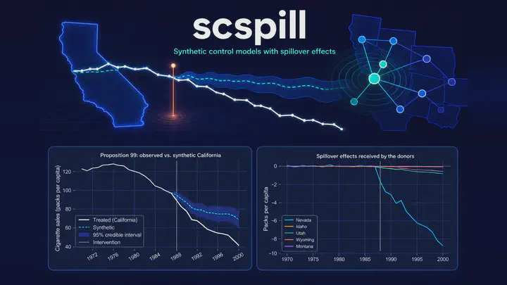
Synthetic control when the treatment leaks — the effect on the treated unit and the spillover received by every donor.

scspill is a Python package of synthetic control models that drop SUTVA on the donor pool. The treatment is allowed to reach the controls, and every model reports two estimands: the effect on the treated unit, purged of the contamination, and the spillover effect received by each donor — something classical synthetic control cannot express at all. The model available today, sar, routes spillovers through spatial weights you supply, scaled by a single intensity ρ that is estimated rather than assumed; it fits unconstrained horseshoe-shrunk synthetic weights, so donors may be dropped, enter negatively, or extrapolate, and it returns full Bayesian uncertainty for both estimands. At ρ = 0 it collapses exactly to the Bayesian horseshoe synthetic control. The estimator architecture follows mlsynth — a pydantic config in, a standardized results object out — and the method names match its SPILLSYNTH dispatcher, so the two libraries compose naturally.

🚀 Get started

Fit a model on California’s Proposition 99 in about ten lines: the ATT with a 95% credible interval, the spillover intensity ρ, the year-by-year spillover received by every donor, MCMC diagnostics, and counterfactual plots.

▶ Open in Colab

🧬 Models

One model ships today: sar, the Bayesian spatial-autoregressive spillover SCM of Sakaguchi & Tagawa (2026). Three further spillover-aware models are on the roadmap — Cao & Dowd, the inclusive SCM of Di Stefano & Mellace, and the partial-interference SCG of Grossi et al. They are not implemented, and SCSPILLConfig rejects their names rather than falling back silently.

🧪 Validation

Evidence that the sar sampler is correct: the Geweke (2004) joint distribution test, prior-sensitivity grids, prior predictive checks, and cross-validation against the authors’ frozen R credible intervals.

What’s inside

scspill — the model layer. SCSPILL(config).fit() returns the ATT and its credible interval, the counterfactual path, the ρ posterior, a time-by-donor spillover panel, and MCMC diagnostics.

scspill.validation — sar’s sampler validation: the Geweke joint distribution test, prior-sensitivity grids, and prior predictive checks.

scspill.simulate — sar’s Monte Carlo engine: a rook-lattice SAR data-generating process and the SCM / BSCM / SCSPILL comparison behind Tables 1–2 of the paper.

scspill.data — the bundled spillover panels below. They are model-agnostic, so any model added later can use them unchanged.

sar is validated, not just implemented — it is cross-validated against the authors’ R replication package: the California and Sudan posteriors against the frozen R credible intervals, the Monte Carlo grid against the paper’s frozen tables, and the prior predictive statistics to three decimals. The defaults are paper-correct: several documented bugs of the reference implementation are fixed, each with an escape hatch or a benchmark quantifying the difference — see the sar model page.

Bundled case studies

scspill.data ships two ready-to-estimate datasets:

• California — Proposition 99, 39 states (1970–2000): per-capita cigarette sales with rook-contiguity weights, via scspill.data.load_california().
• Sudan — the 2011 secession, 34 African countries (2000–2015): GDP per capita with trade-network weights, via scspill.data.load_sudan(). Worked through in the Sudan case study.

Installation

Install the latest release from PyPI (the core install is pure NumPy/SciPy; the numba extra adds JIT-compiled samplers):

pip install scspill              # NumPy/SciPy sampler backend
pip install "scspill[numba]"     # + JIT-compiled samplers (~10x faster)
pip install "scspill @ git+https://github.com/quarcs-lab/scspill.git"   # latest

Requires Python 3.10+.

At a glance

Load a bundled case study, fit the sampler, and read off both estimands:

from scspill import SCSPILL
from scspill.data import load_california

panel = load_california()        # Prop 99 panel + rook-contiguity weights
result = SCSPILL(
    {**panel.config_kwargs(), "m_iter": 20_000, "burn": 10_000, "seed": 42}
).fit()

result.att, result.att_ci          # treatment effect on California + 95% CrI
result.rho_hat, result.rho_ci      # spillover intensity posterior
result.spillover_panel["Nevada"]   # the effect received by Nevada, per year
result.diagnostics()               # ESS / R-hat / MCSE per chain
result.plot(kind="panel")          # counterfactual | effect | top spillovers

Head to Get started, Models and Validation to see the estimators in action.

Built on

scspill keeps its dependencies deliberately light — the modern Python scientific stack, and nothing else:

• NumPy and SciPy — the sampler backend
• pandas — panels and the spillover tables
• pydantic — the validated estimator configuration
• matplotlib — the diagnostic and counterfactual figures
• numba — optional JIT-compiled samplers

Acknowledgement

The Python package is written and maintained by Carlos Mendez. The sar model and its original R/C++ implementation are the work of Shosei Sakaguchi and Hayato Tagawa — please cite their article whenever you fit that model. Their replication package is MIT-licensed, its copyright notice is retained in the library’s LICENSE, and every release of scspill is cross-validated against its frozen results. The estimator architecture follows Jared Greathouse’s mlsynth; the documentation stack follows the QuaRCS Lab’s geometrics package.

If you use scspill, please cite both the software and the methodological article (machine-readable metadata lives in CITATION.cff):

Mendez, C. (2026). Synthetic Control Models with Spillovers in Python (version 0.2.1). https://github.com/quarcs-lab/scspill

Sakaguchi, S., & Tagawa, H. (2026). Identification and Bayesian Inference for Synthetic Control Methods with Spillover Effects. The Econometrics Journal. https://doi.org/10.1093/ectj/utag006

Released under the MIT license.