WebApps

Runnable concept sandboxes and plain-language explanations of spatial convergence and inequality methods.

Map and describe regions: choropleths, spatial weights, Moran scatterplots, LISA cluster maps and space-time views.

Estimate beta-, sigma- and club convergence, spatial econometric models, Markov dynamics, Gini/Theil inequality and (M)GWR.

Runnable concept sandboxes and plain-language explanations of panel-data methods.

Describe and visualize a panel: distributions, missing values, time trends, within/between variation and panel dynamics.

Estimate fixed, random and correlated random effects, FWL, Hausman tests, event studies, convergence and Kuznets waves.

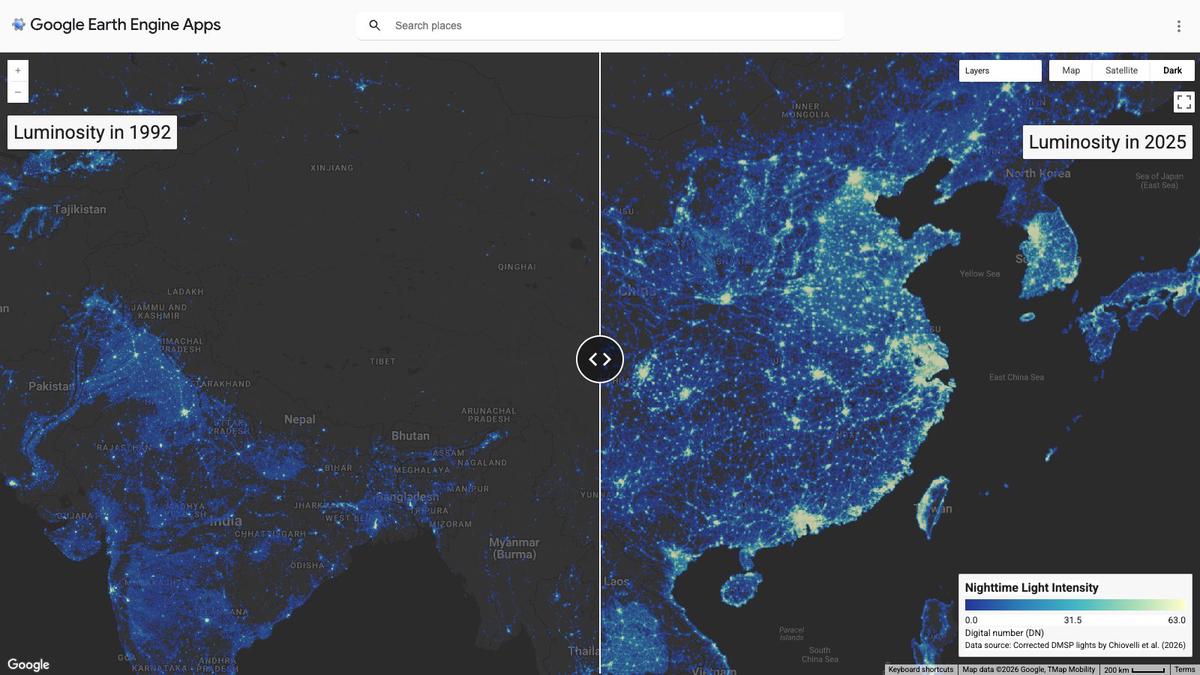
Interactive Google Earth Engine application.

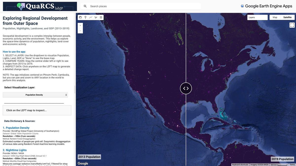
Interactive Google Earth Engine application.

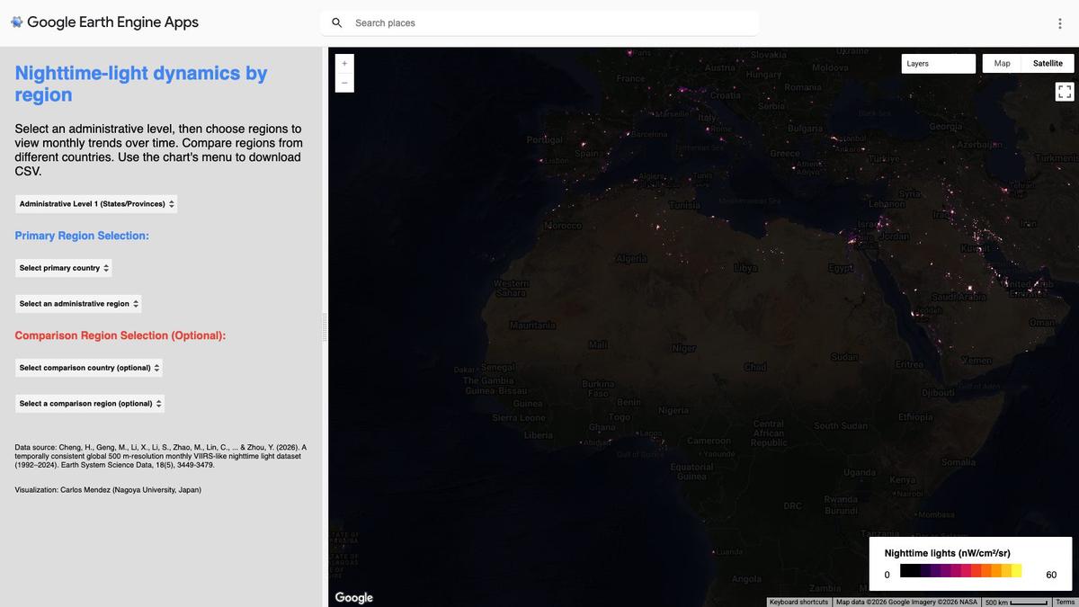
Interactive Google Earth Engine application.

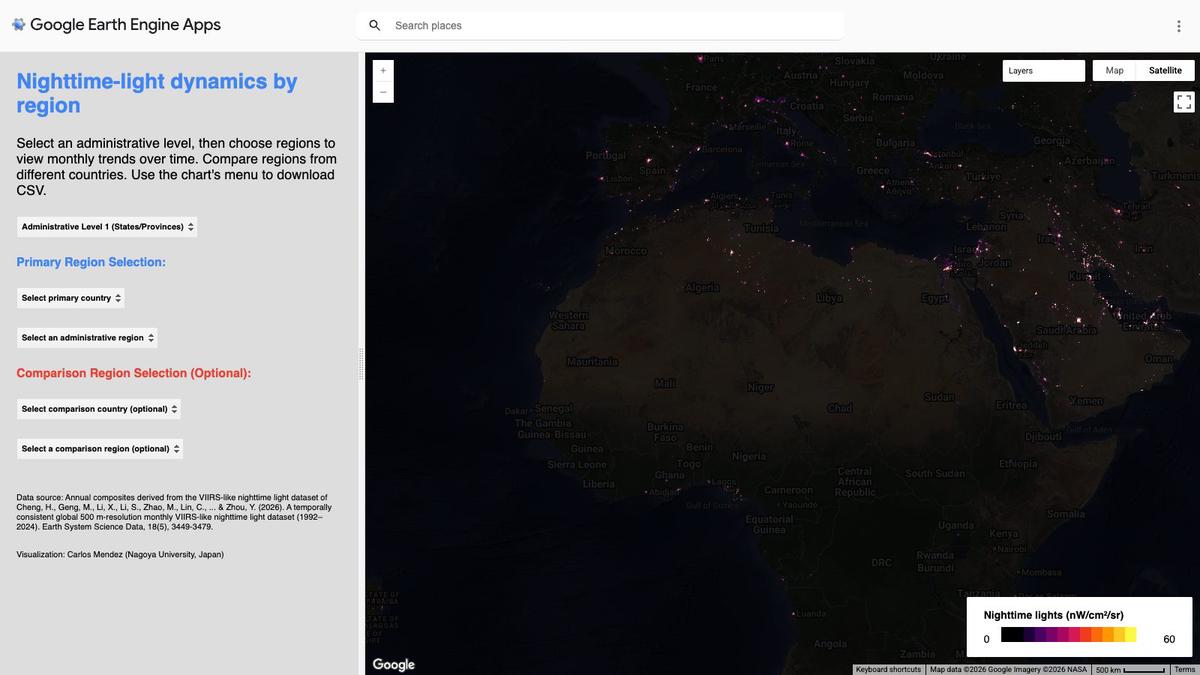
Interactive Google Earth Engine application.

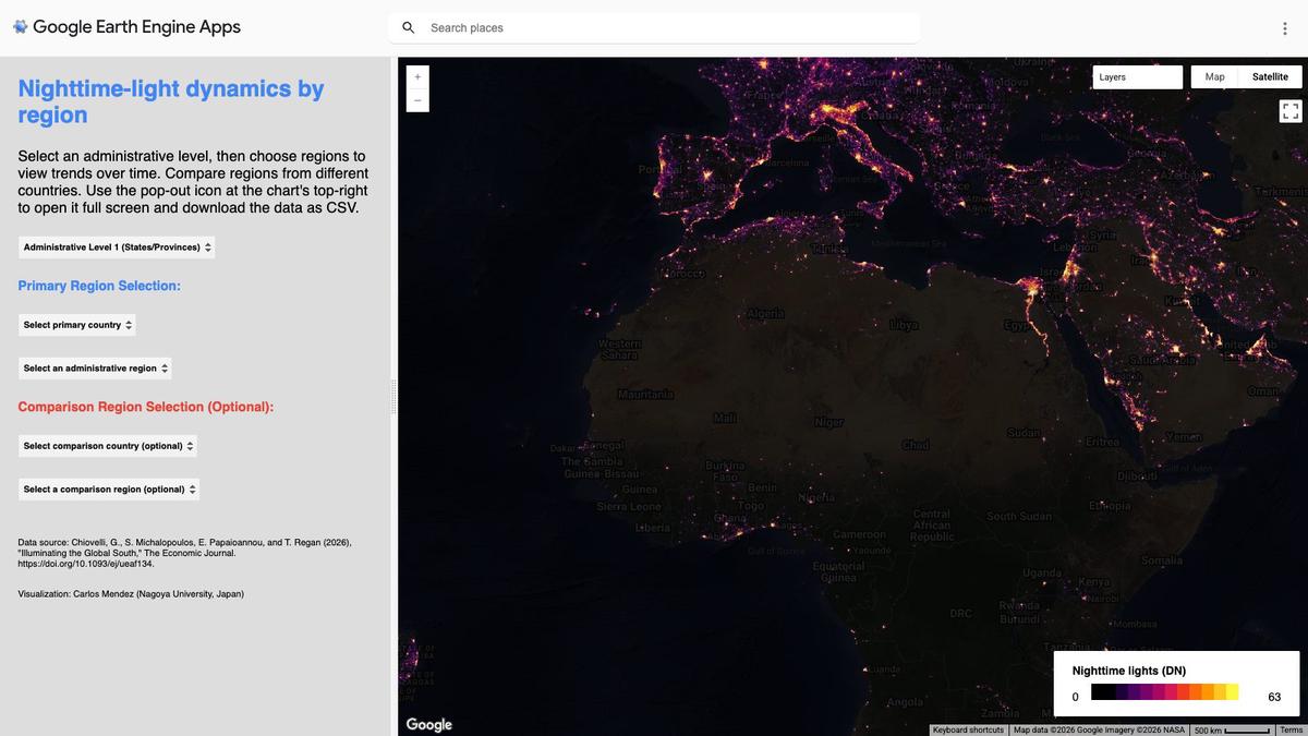
Interactive Google Earth Engine application.

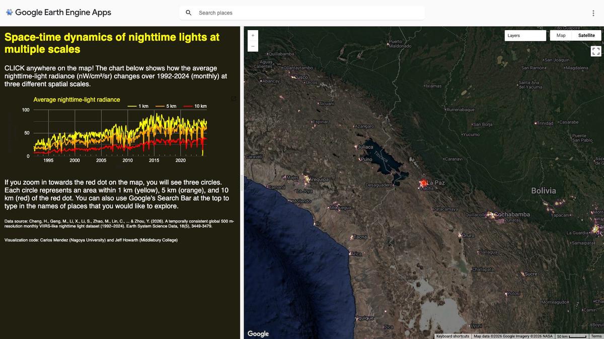
Interactive Google Earth Engine application.

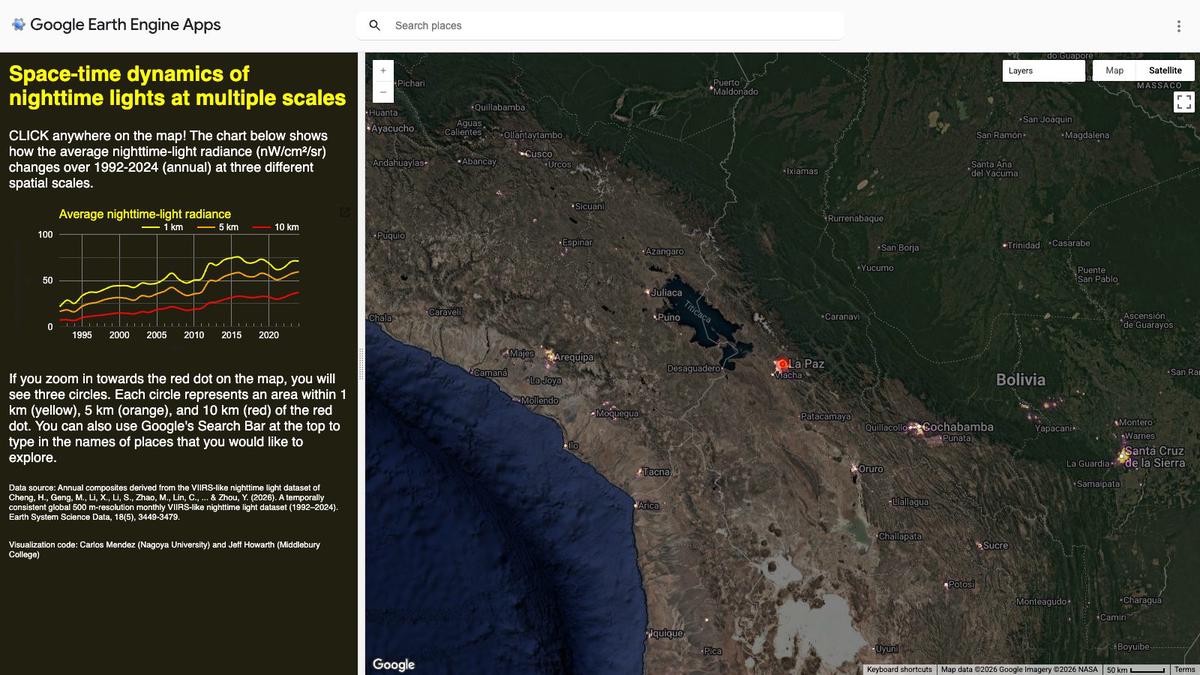
Interactive Google Earth Engine application.

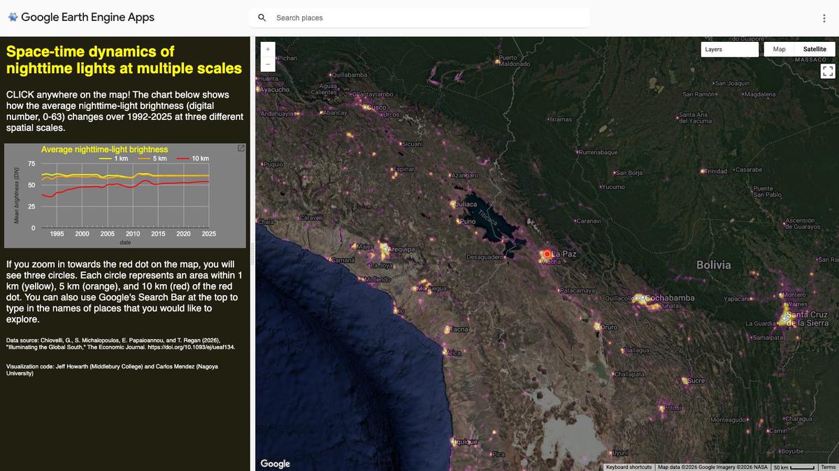
Interactive Google Earth Engine application.

Interactive Google Earth Engine application.

Interactive Google Earth Engine application.

Interactive Google Earth Engine application.

Interactive Google Earth Engine application.

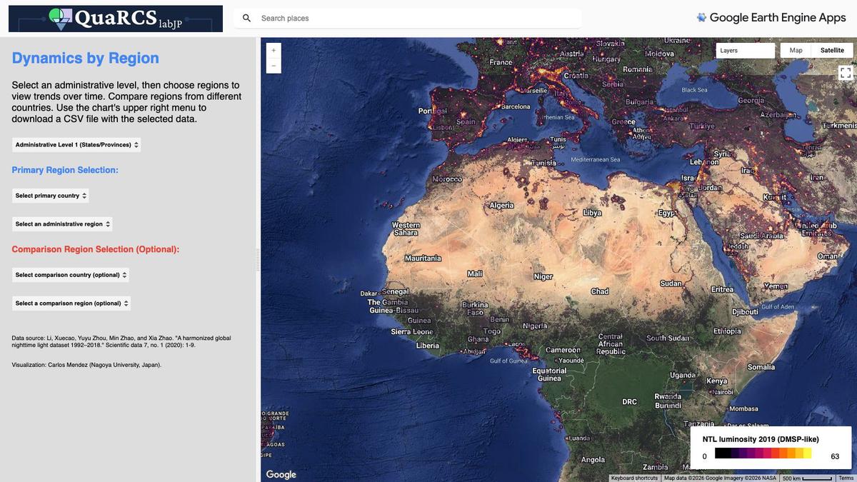
Interactive Google Earth Engine application.

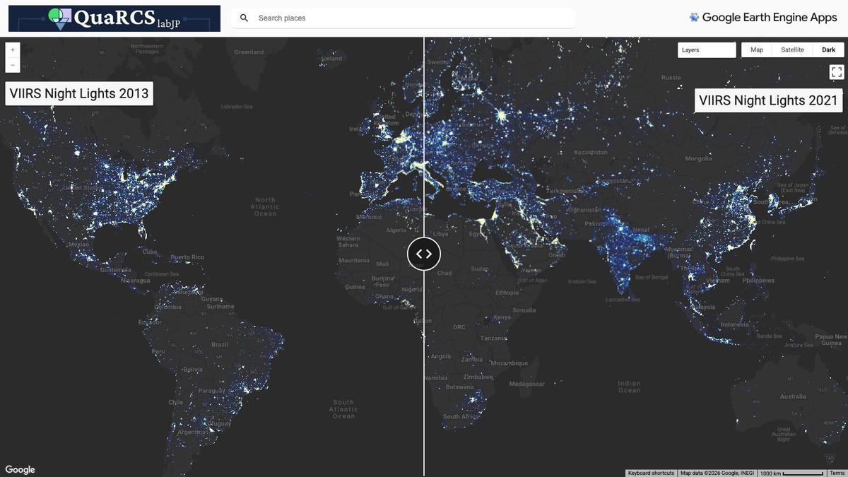
Interactive Google Earth Engine application.

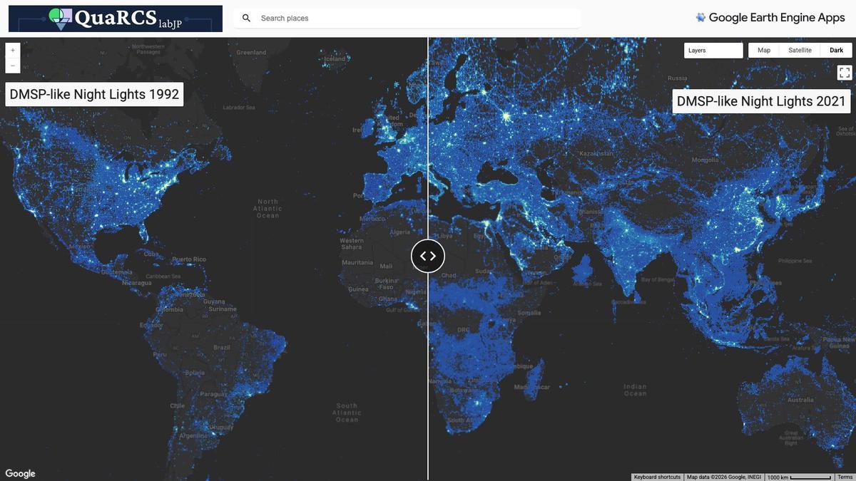
Interactive Google Earth Engine application.

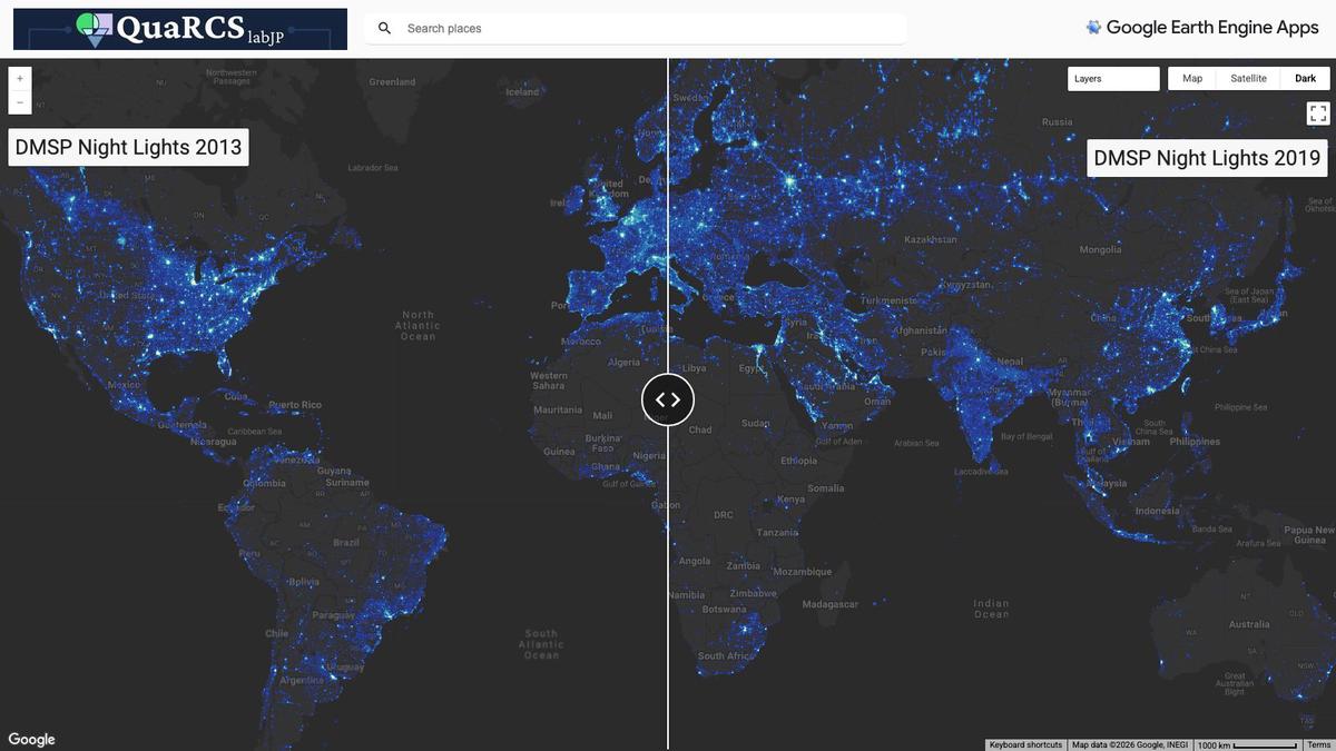
Interactive Google Earth Engine application.

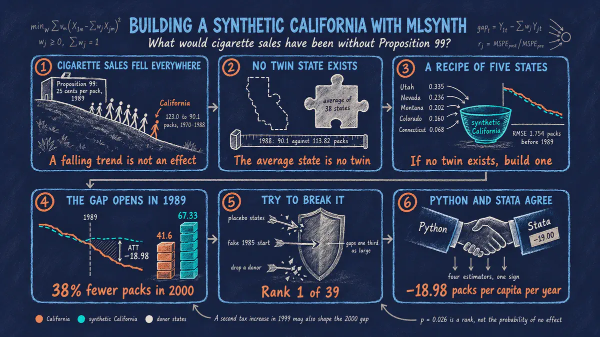
Learn the synthetic control method and the mlsynth library in Python with the Proposition 99 tobacco case. The tutorial builds a synthetic California from five donor states and reads its weights and predictor balance. It tests the result with in-space and in-time placebos and leave-one-out refits, replicates the Stata edition, and compares four mlsynth estimators.

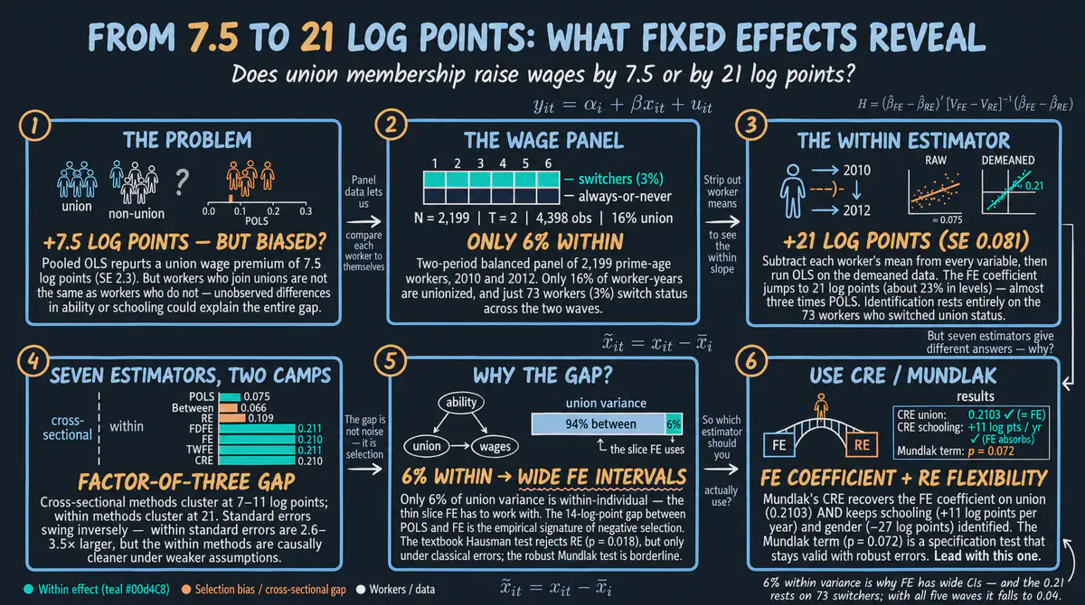
A beginner-friendly tour of seven panel-data estimators, from pooled OLS to correlated random effects (Mundlak), applied to a two-period worker wage panel. Predict-first checks, two short proofs, an interactive lab, and worked exercises show why the within estimators nearly triple the union wage premium.

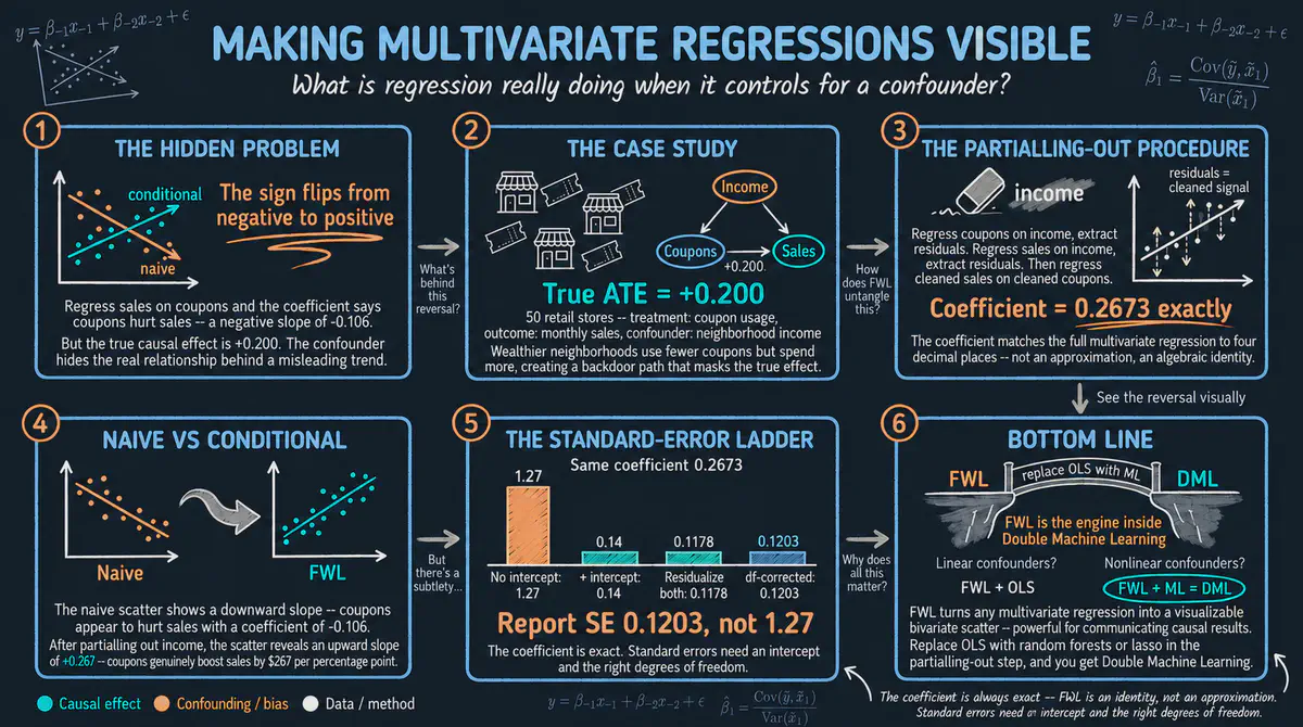
Understanding the Frisch-Waugh-Lovell theorem to isolate causal relationships by partialling-out confounders in a simulated fast-food coupon promotion, with an appendix that extends FWL to panel data

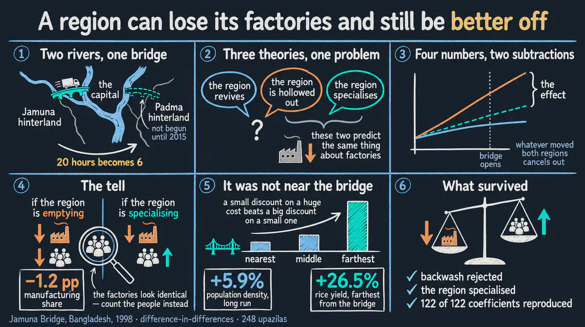
In June 1998 a 4.8-kilometre bridge over the Jamuna river connected 26 million isolated Bangladeshis to Dhaka and cut freight costs in half. This tutorial rebuilds the difference-in-differences evaluation of that bridge from the ground up in Python, using the Padma hinterland — a symmetric region left isolated by a river whose own bridge was not started until 2015 — as the comparison group. It teaches the 2x2 logic, parallel trends, two-way fixed effects, event studies and honest sensitivity analysis on satellite nighttime lights, then runs the same machinery over census employment shares, rice yields and a public-goods placebo. The two doubly robust estimators of the original paper are rebuilt by hand in NumPy and pushed through both diff-diff and pyfixest. All 122 published coefficients are audited side by side with the replication, and the defects found inside the shipped Stata package are documented in full.

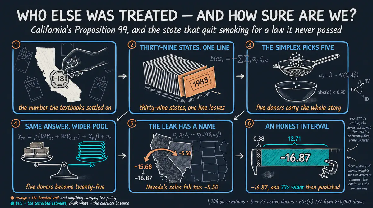
A ground-up introduction to synthetic control in Python, built on the California Proposition 99 case study and climbing three stages: the classical simplex of Abadie, Diamond and Hainmueller; a Bayesian horseshoe prior that lets the data rather than a constraint choose the donors; and the Bayesian spatial model of Sakaguchi and Tagawa, which drops SUTVA on the donor pool and asks who else was treated. Every equation is derived and mapped to the code that implements it, using the scspill and mlsynth libraries. The answer for California survives every relaxation. The claim that the donor pool was clean does not.

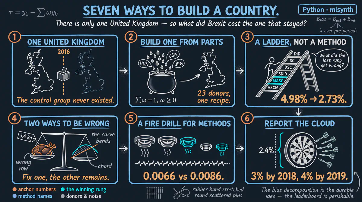
A careful introduction to mlsynth, the Python library that puts the whole family of single-treated-unit synthetic control estimators behind one configuration interface. We climb the ladder from difference-in-differences to synthetic difference-in-differences with one mlsynth class per stage, showing what every option does and where the defaults will quietly hand you a different estimator. The case study is the 2016 Brexit referendum and what it cost UK GDP.

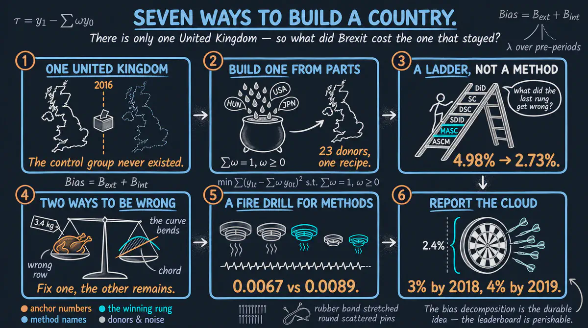
Climbing the ladder from difference-in-differences to synthetic difference-in-differences, one stage at a time, with every estimator hand-coded before it is run with its package. The case study is the 2016 Brexit referendum and what it cost UK GDP. Includes cheat sheets in R, Stata and Python.

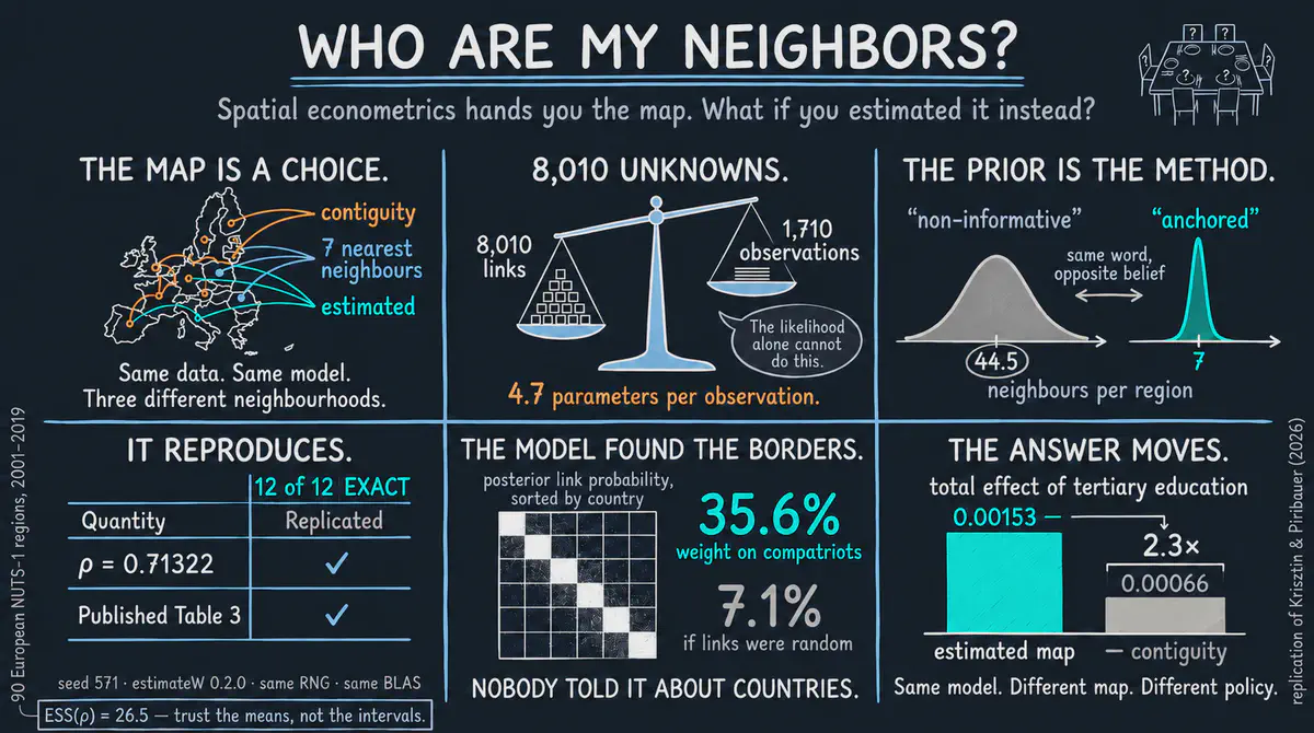
Spatial econometrics usually hands you the neighborhood map before you start. This tutorial estimates it from the data instead, using the estimateW package on 90 European NUTS-1 regions, 2001-2019.

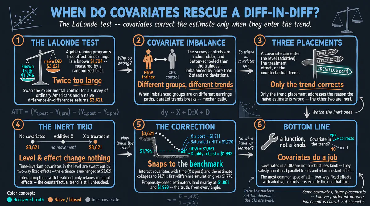
Reproducing Scott Cunningham’s LaLonde test in Python — covariates rescue a difference-in-differences ATT only when they enter the control group’s counterfactual trend, recovering the $1,794 experimental benchmark from a naive $3,621.

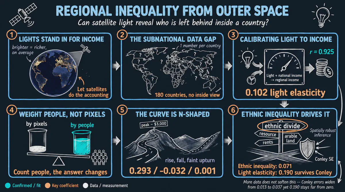
A comprehensive, beginner-friendly Python replication of Lessmann and Seidel (2017) — turning satellite nighttime lights into predicted regional GDP, building five population-weighted inequality indices from scratch, exploring the cross-country dynamics of regional inequality, and estimating the regional Kuznets curve, its determinants, and a Conley spatial-HAC robustness check with PyFixest.

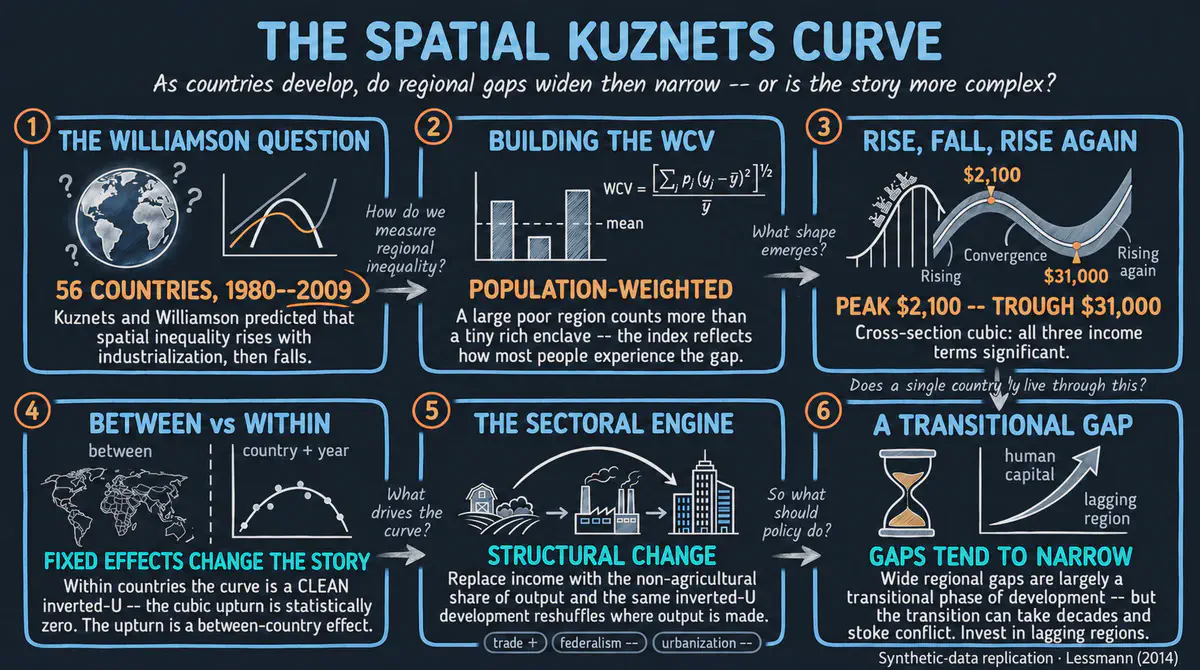
A beginner-friendly R replication of Lessmann (2014) on the spatial Kuznets curve — building the weighted coefficient of variation from simulated regional data, then estimating the inverted-U with cross-section OLS, two-way fixed effects in fixest, and the Robinson and Baltagi–Li semiparametric estimators.

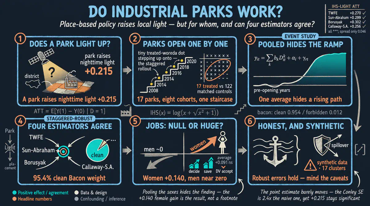
Do industrial parks raise local economic activity — and for whom? A beginner’s staggered difference-in-differences evaluation of Ethiopian industrial parks in Python, replicating Huang, Wang & Xu (2026) on synthetic calibrated data: TWFE and an event study with pyfixest, the modern Sun-Abraham, Borusyak/Gardner and Callaway-Sant’Anna estimators plus a Goodman-Bacon decomposition with diff-diff, survey-weighted repeated-cross-section DiD on DHS household welfare and women’s empowerment, and Conley spatial standard errors.

How persistent is firm employment? Pooled OLS, fixed effects, Anderson-Hsiao IV, Arellano-Bond difference GMM, and Blundell-Bond system GMM on the classic 140-firm UK panel — and how the AR(2), Hansen, and instrument-collapse diagnostics separate the one defensible estimate from four seductive wrong ones.

Evaluate the long-run economic impact of a localized natural disaster with causal inference in Python. A beginner’s replication of Heger & Neumayer (2019) on the 2004 Aceh tsunami, using synthetic calibrated data: dynamic difference-in-differences with pyfixest, an event study with diff-diff, a night-lights dose-response, synthetic control with mlsynth, and Conley spatial standard errors.

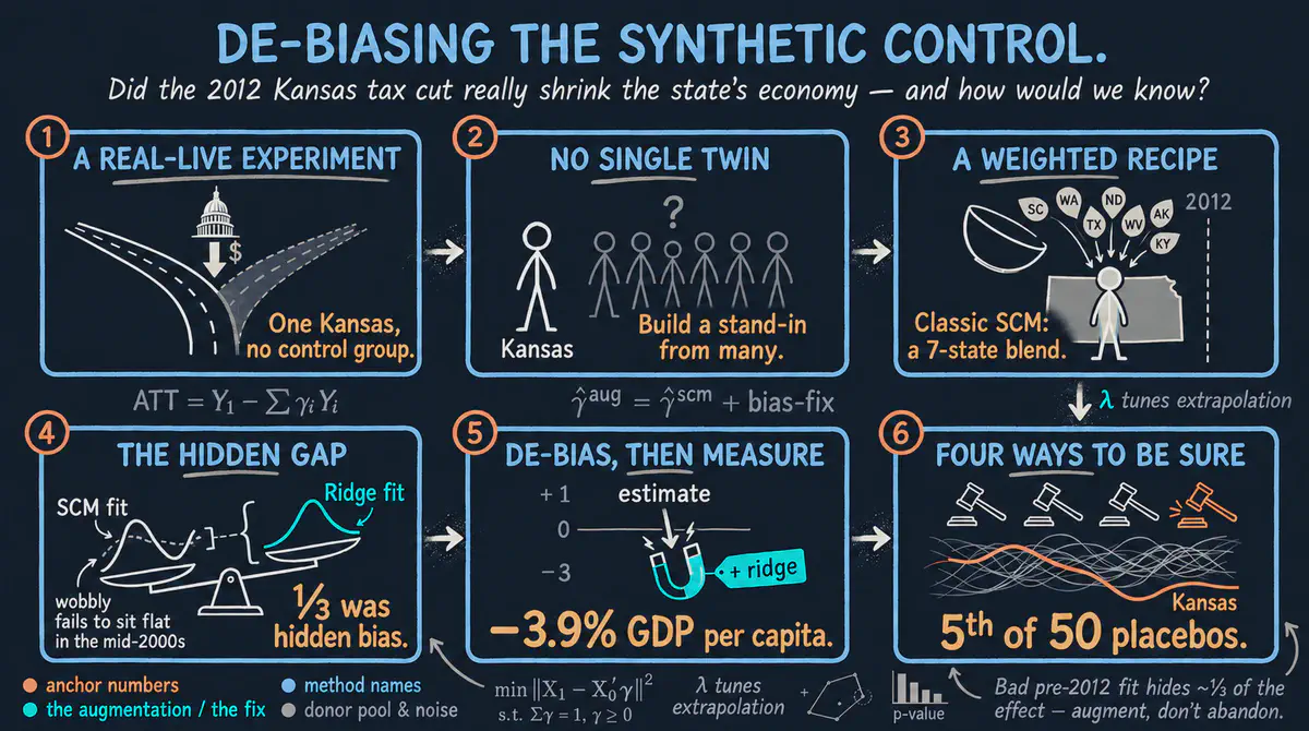
A beginner-friendly, intuition-first tutorial on the Augmented Synthetic Control Method (ASCM) for a single treated unit — estimating the effect of the 2012 Kansas tax cuts on GDP per capita with the augsynth package, from classic SCM to ridge augmentation, with a careful tour of four ways to do inference.

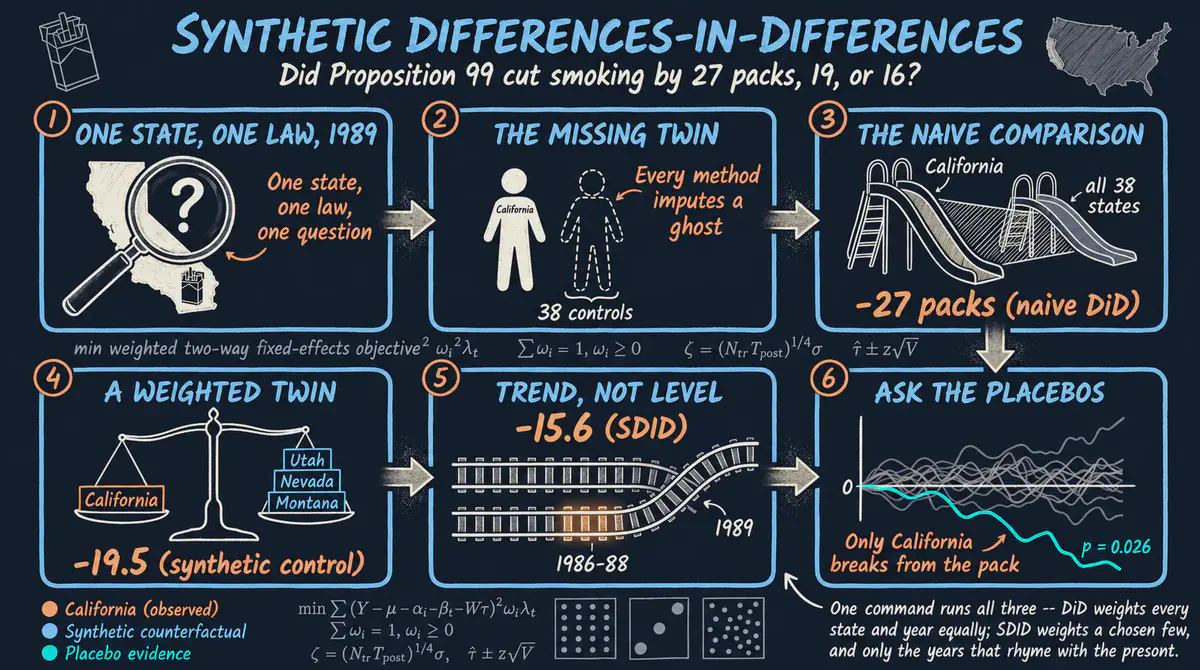
Introduce and derive synthetic difference-in-differences, then apply it to California’s Proposition 99 — comparing SDID with the original difference-in-differences and synthetic control (synth2), and how to run placebo inference with a single treated unit.

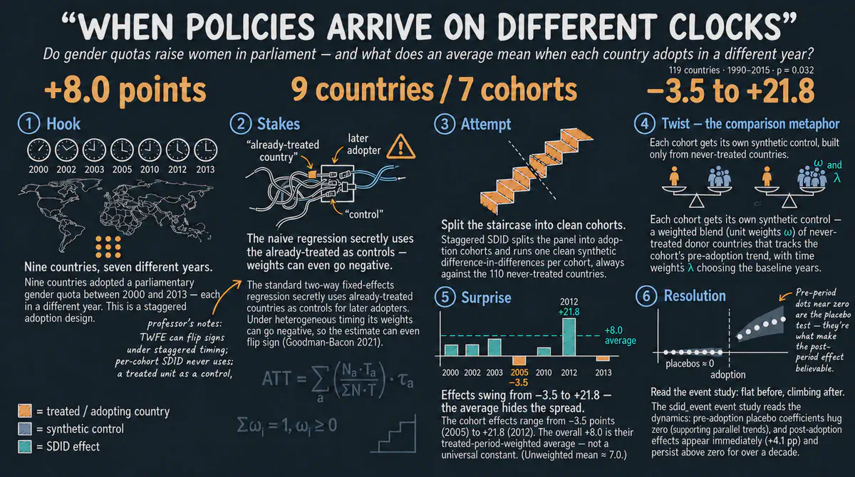
Extend synthetic difference-in-differences to staggered adoption, where units adopt treatment at different times, and apply it in Stata to parliamentary gender quotas across 119 countries — deriving the per-cohort estimator, its aggregation into the overall ATT, the modern sdid_event event study, and bootstrap, jackknife, and placebo inference.

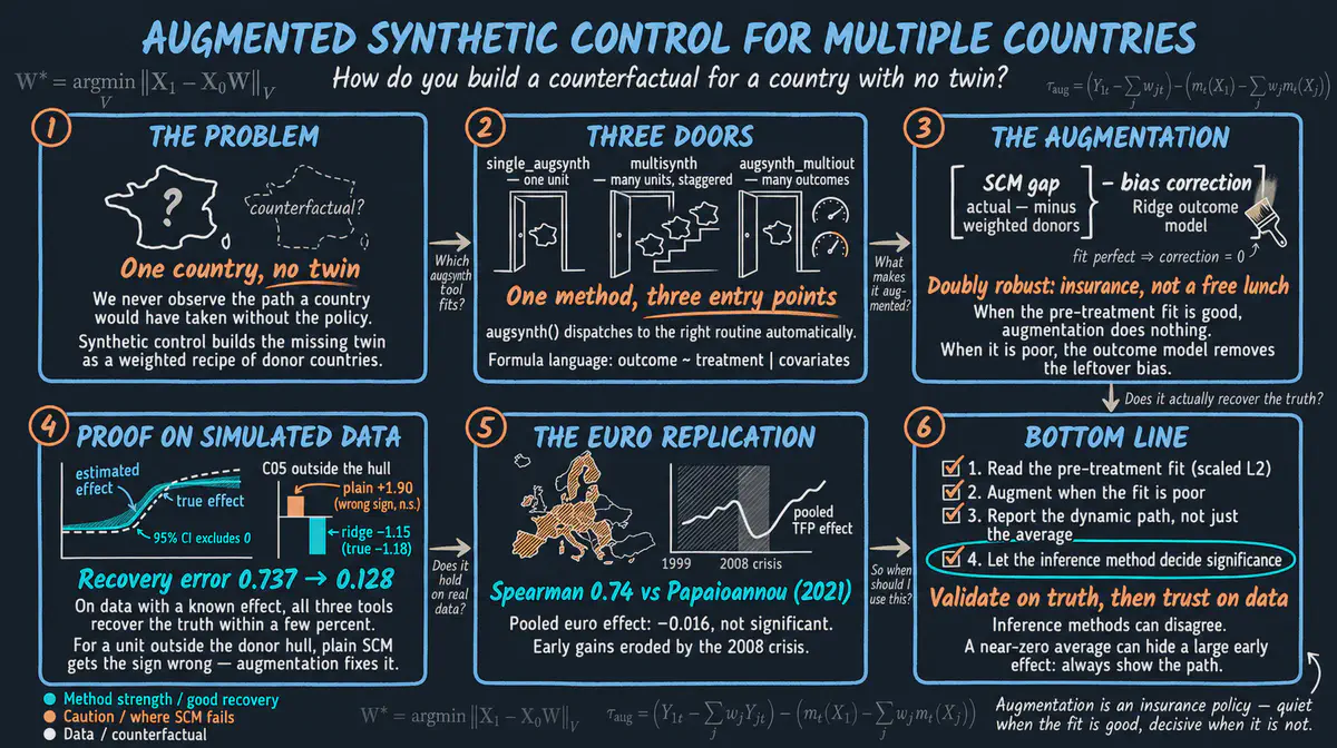
A hands-on tour of the Augmented Synthetic Control Method in a multi-country setting with the augsynth package — learning single_augsynth, multisynth, and augsynth_multiout on simulated data, then replicating Papaioannou (2021) on the EMU and productivity convergence.

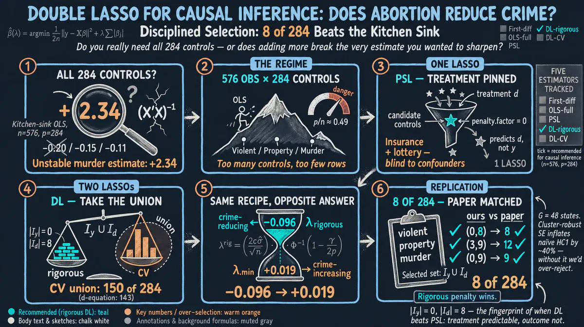
A beginner-friendly walkthrough of Double LASSO for causal inference, replicating Fitzgerald, Lattimore, Robinson and Zhu’s (2026) analysis of the Donohue–Levitt abortion–crime question with 284 candidate controls and state-clustered standard errors.

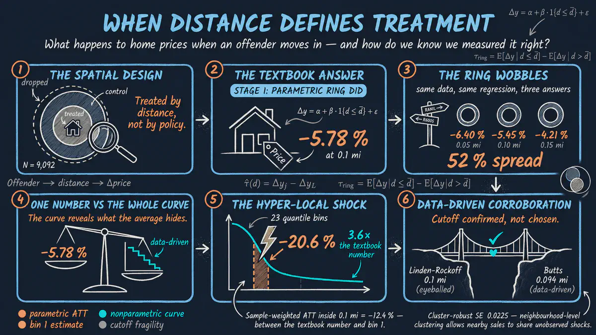
When the ’treatment’ is a point in space, distance becomes the running variable. We walk through the parametric ring DiD and a data-driven nonparametric alternative, first on a simulated world with a known answer, then on Linden and Rockoff’s home-prices study, and reconcile a parametric −5.78 % with a nonparametric −20.6 %.

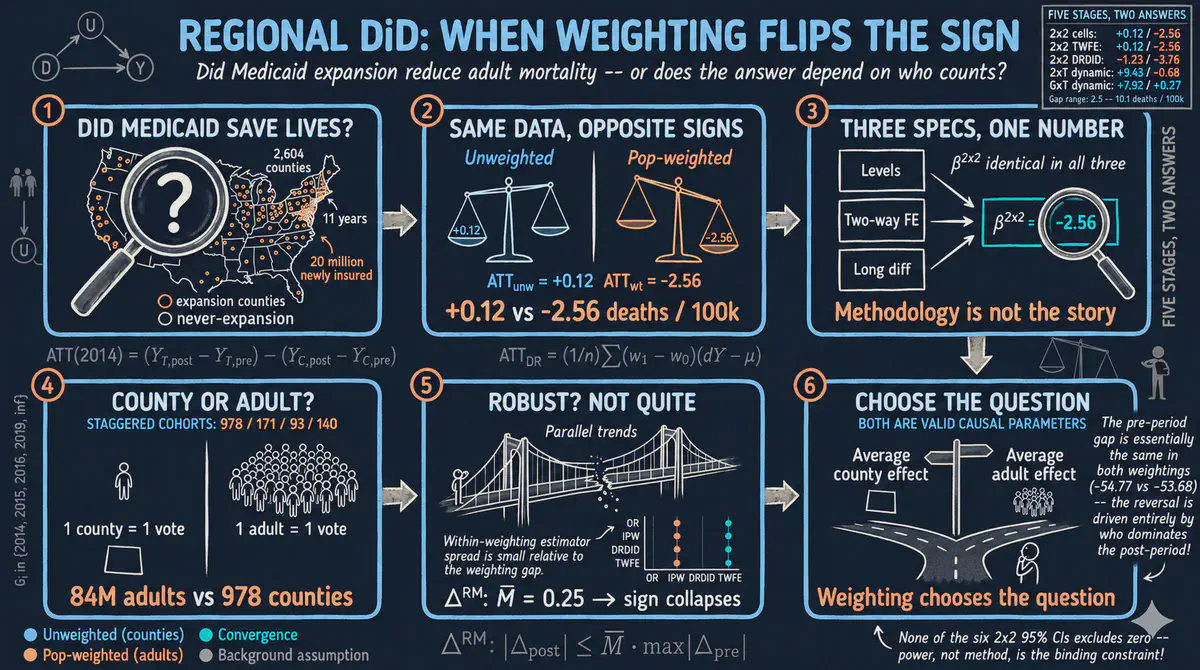
A case study on the Affordable Care Act’s Medicaid expansion — working through 2x2 cell-means, TWFE, covariate-adjusted DRDID, 2xT and Callaway-Sant’Anna staggered event studies, and HonestDiD sensitivity — to show how population weighting changes the target parameter when the units are regions of very different sizes.

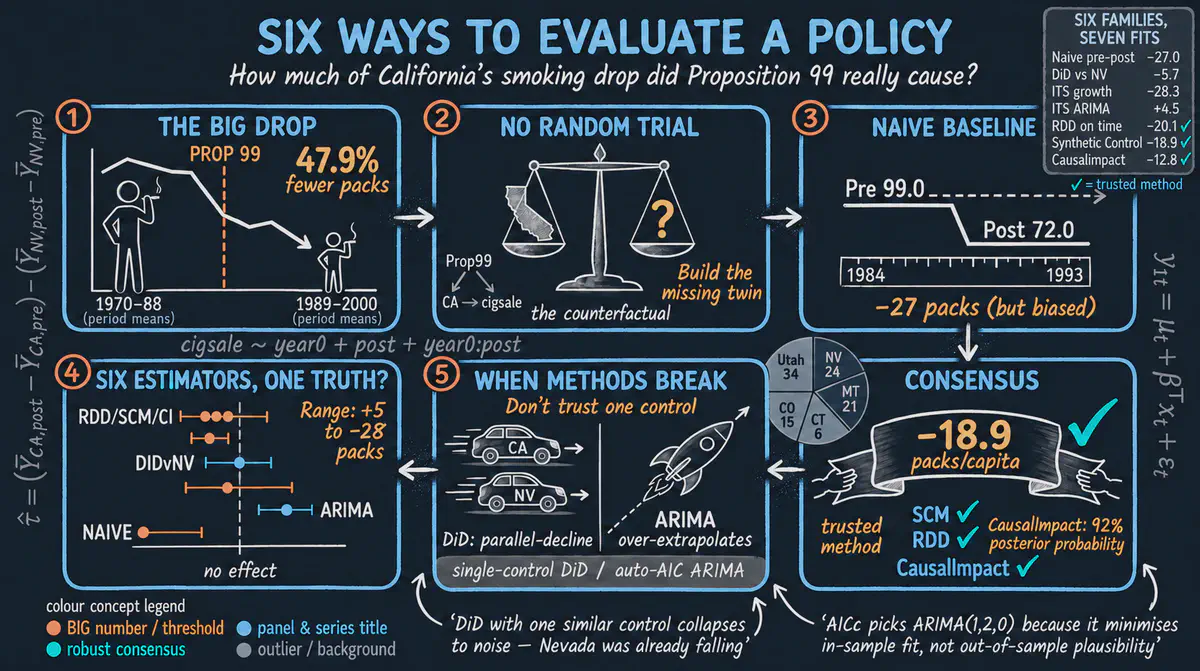
Six estimators in one tutorial — naive pre-post, DiD, two flavours of ITS, RDD on time, Synthetic Control, and CausalImpact — all applied to California’s 1988 Proposition 99 cigarette tax to see how much (and where) they disagree.

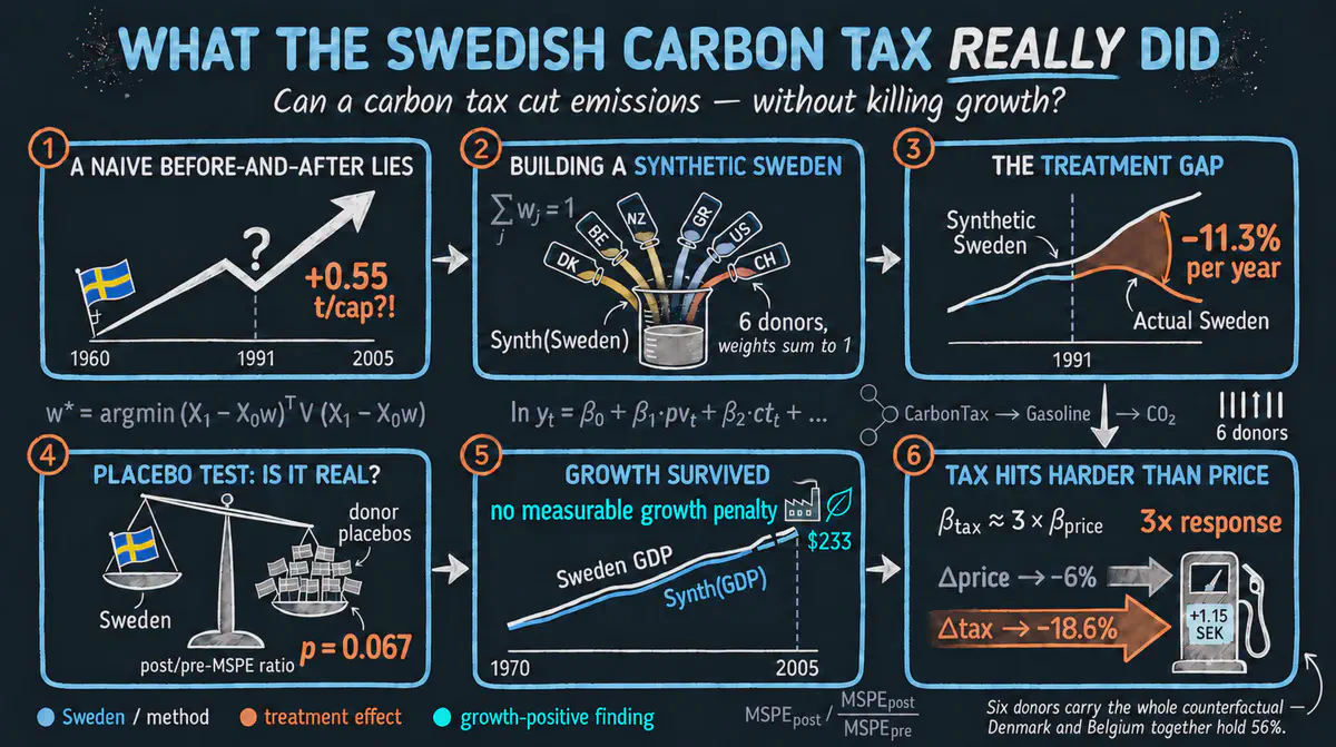
Synthetic Control and IV in Python — replicating Andersson (2019) on Sweden’s carbon tax and CO2 emissions with pysyncon and pyfixest.

Replicating the California tobacco case study from Sakaguchi & Tagawa in R: three estimators, one ATT, and a Nevada-sized spillover.

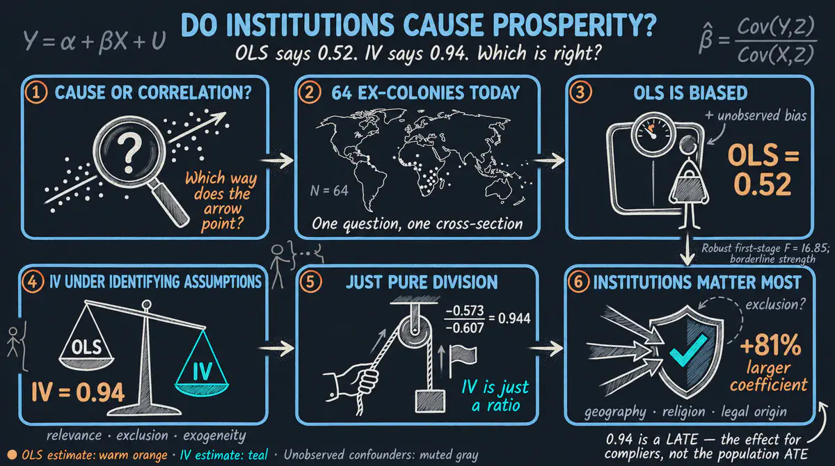
Replicate Acemoglu, Johnson and Robinson (2001) in Python with pyfixest and linearmodels: instrument modern institutions with settler mortality across 64 ex-colonies and learn how IV recovers a causal effect that OLS understates by 80 percent.

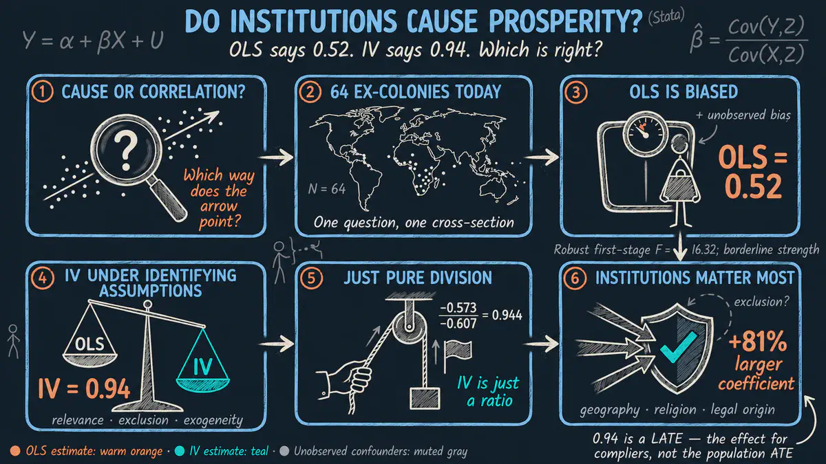
Replicate Acemoglu, Johnson and Robinson (2001) in Stata: instrument modern institutions with settler mortality across 64 ex-colonies and learn how IV recovers a causal effect that OLS understates by 80 percent.

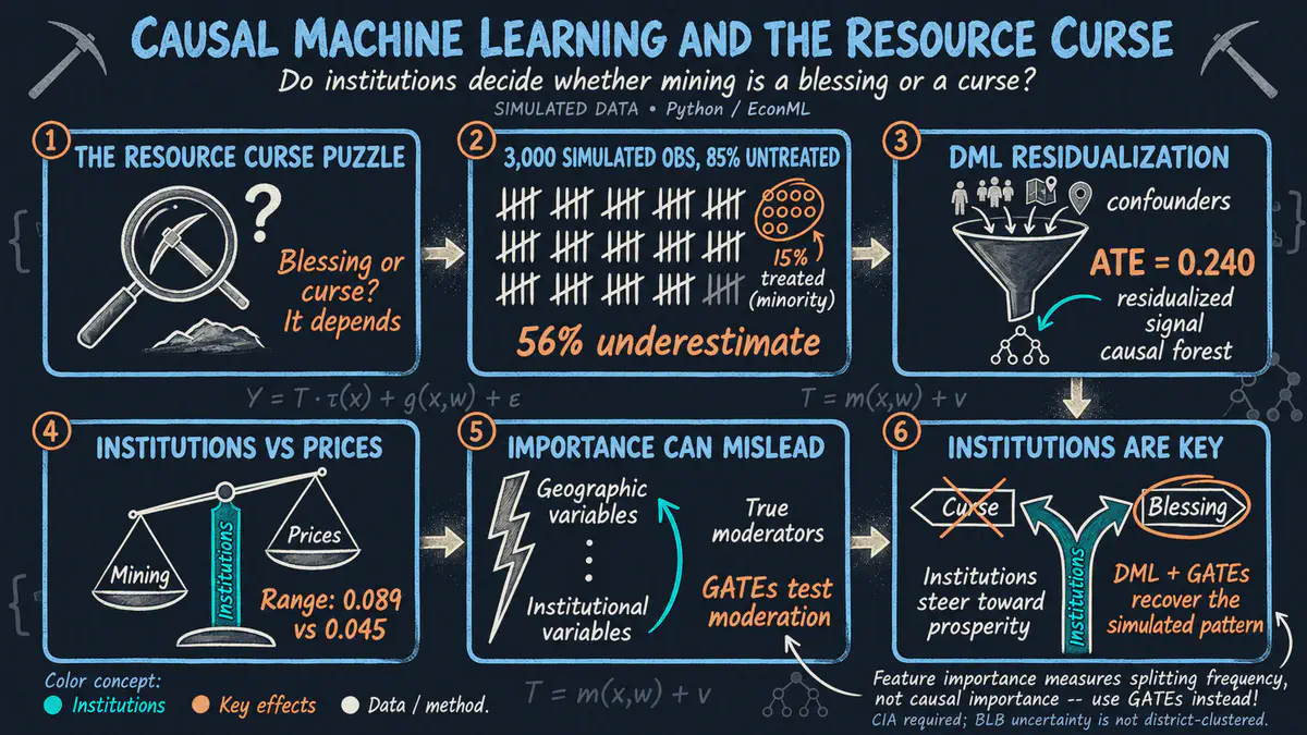
Estimate heterogeneous causal effects of mining and mineral prices on economic development using EconML’s CausalForestDML with Double Machine Learning, applied to simulated resource curse data

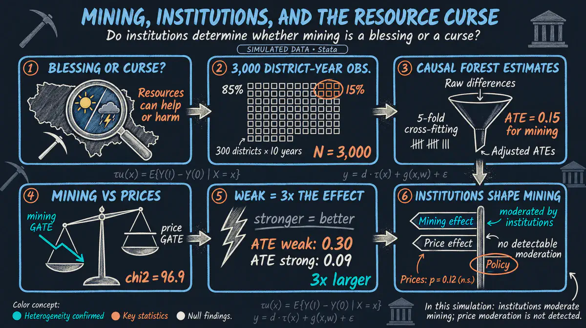
Estimate heterogeneous causal effects of mining and mineral prices on economic development using Stata 19’s cate command with multi-valued treatment via pairwise binary comparisons, applied to a simulated resource curse panel dataset

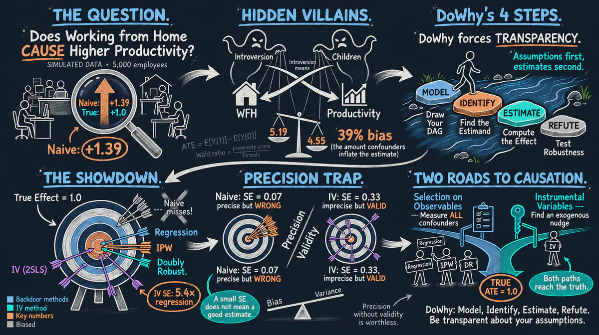
A beginner-friendly introduction to causal inference using DoWhy’s four-step framework with simulated observational data on working from home and productivity

A faithful Python tutorial on Li & Fotheringham (2026) — using a two-stage MGWFER algorithm to remove time-invariant spatial confounders from Multiscale GWR and recover both unbiased spatially varying slopes and intrinsic contextual effects from simulated panel data (225 units x 3 periods).

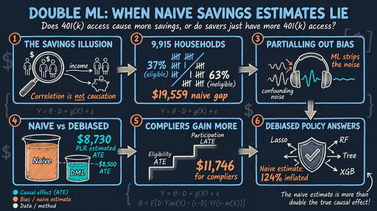
Estimating the causal effect of 401(k) eligibility and participation on net financial assets using three DoubleML models (PLR, IRM, IIVM) with the 1991 SIPP pension dataset

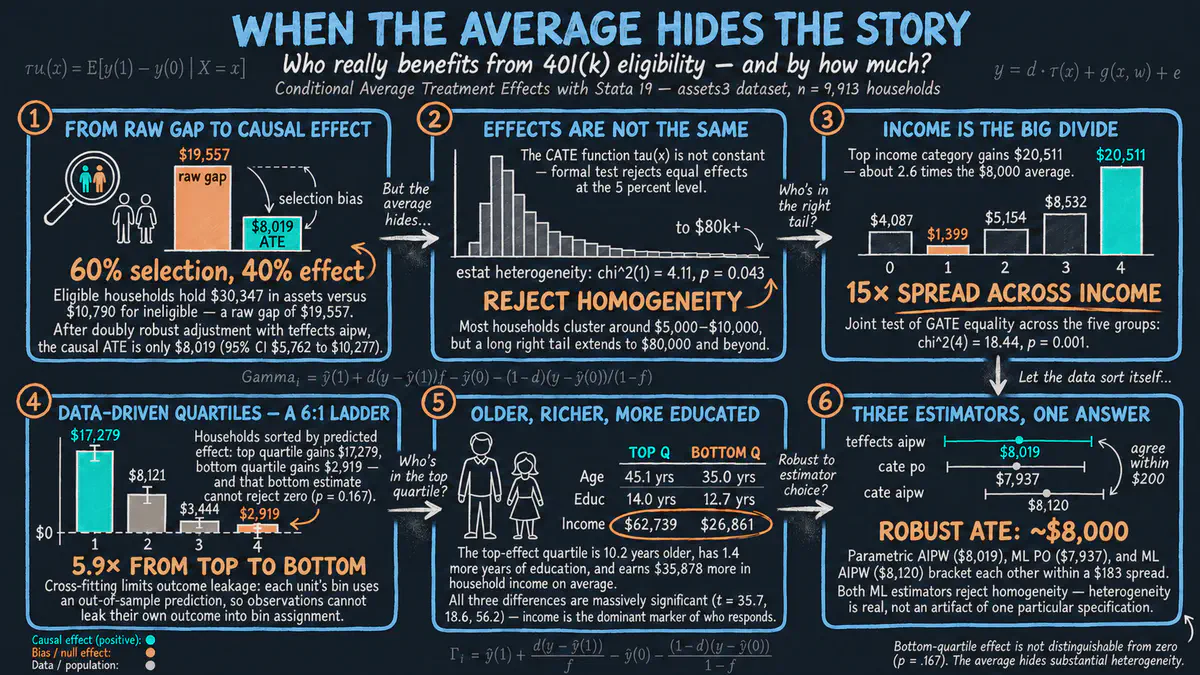
Estimate how the effect of 401(k) eligibility on household assets varies across households using Stata 19’s new cate command, with PO, AIPW, GATE, GATES, and nonparametric series estimators applied to the canonical assets3 dataset

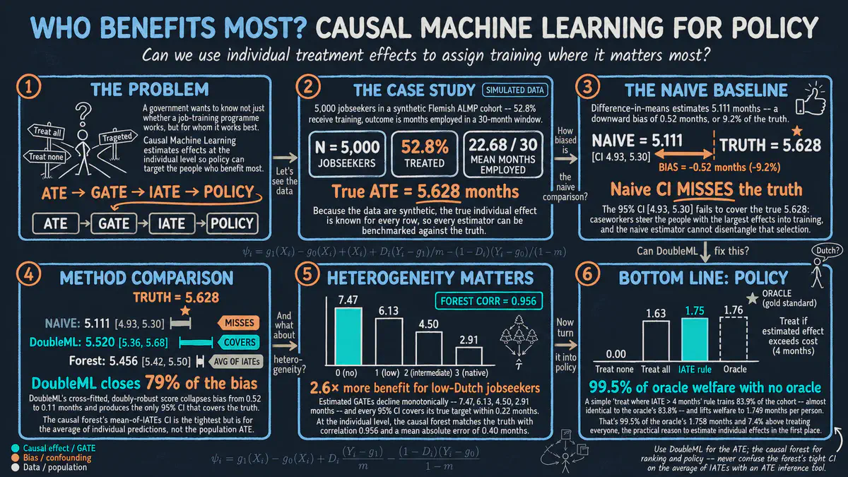
A beginner-friendly walk-through of Causal Machine Learning — ATE, GATE, IATE, and welfare-maximising assignment — using DoubleML and EconML on a synthetic Flanders ALMP-style cohort with known true effects.

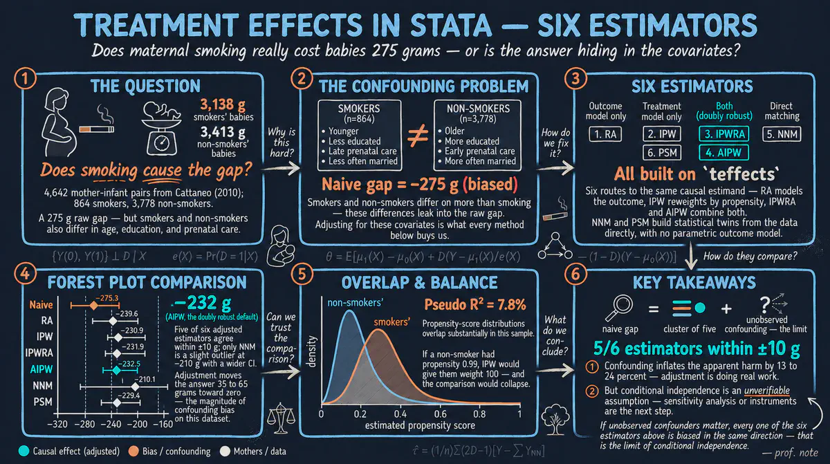
A beginner-friendly walk-through of six treatment-effects estimators in Stata — regression adjustment, IPW, IPWRA, AIPW, nearest-neighbor matching, and propensity-score matching — applied to the classic maternal-smoking and birth-weight case study.

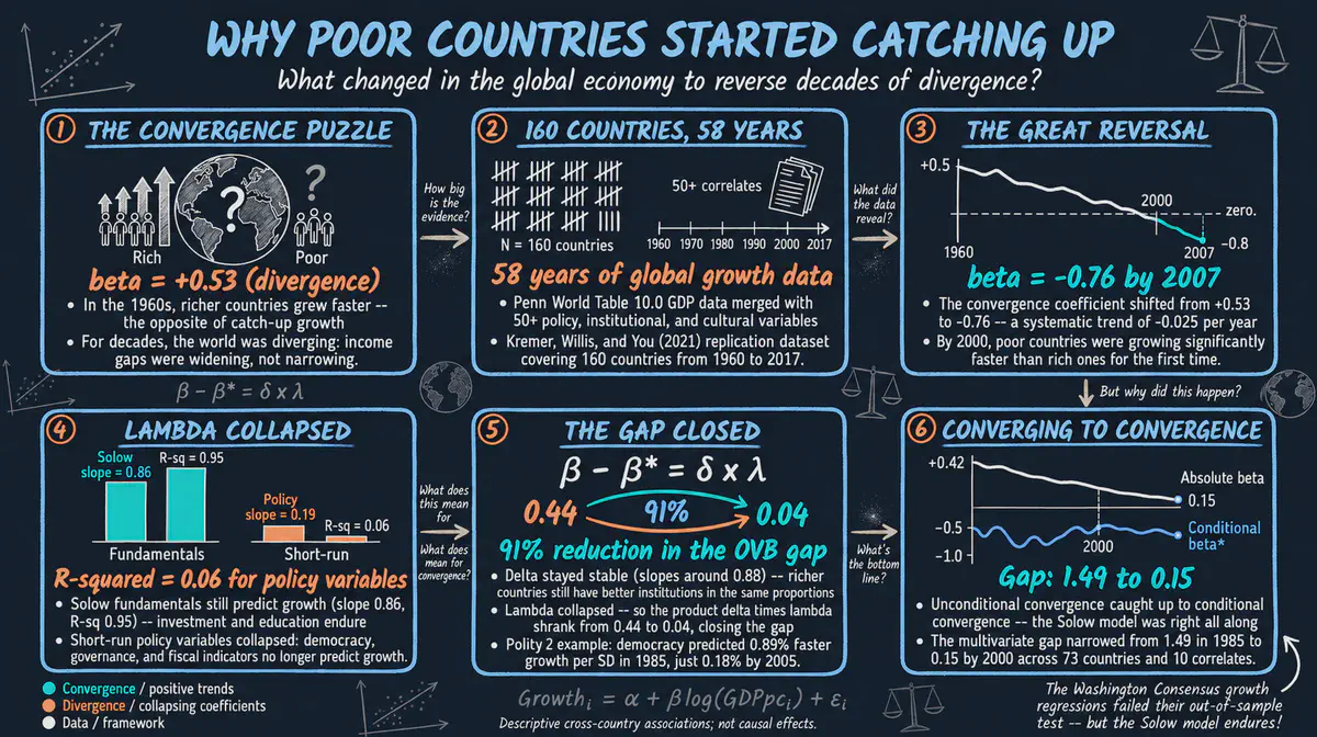
Reproduce the key findings of Kremer, Willis, and You (2021) to understand why unconditional convergence emerged since 2000 and how the convergence of growth correlates explains this shift

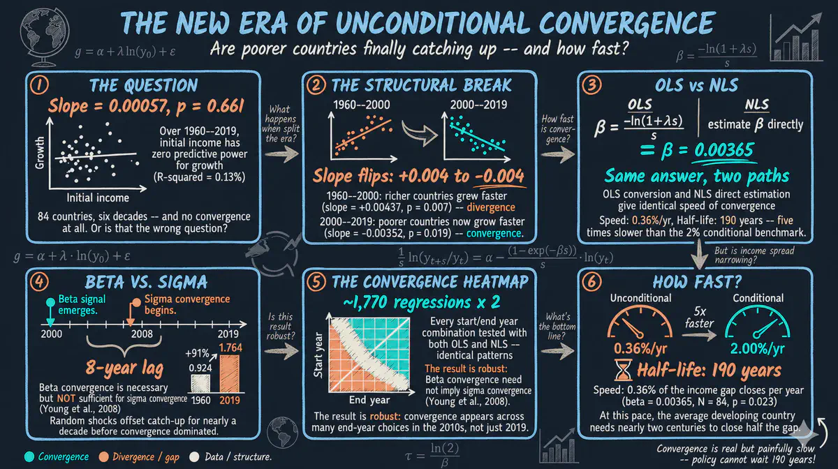
Test whether poorer countries are catching up to richer ones using beta and sigma convergence analysis with Penn World Tables 10.0 data in Stata

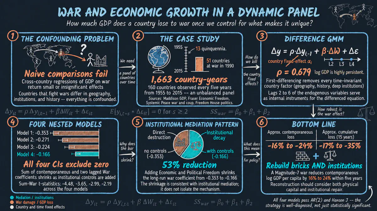
Estimate the within-country dynamic effect of war on log GDP per capita using Arellano-Bond GMM in Stata, reproducing Thies and Baum (2020) on a 1955-2015 panel of 160 countries.

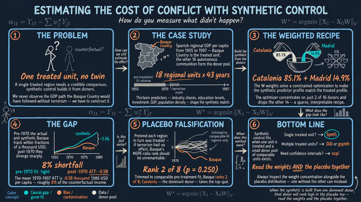
A beginner-friendly tutorial on the synthetic control method in R, using the Basque Country case study to estimate the economic cost of conflict on regional GDP per capita from 1970 to 1997.

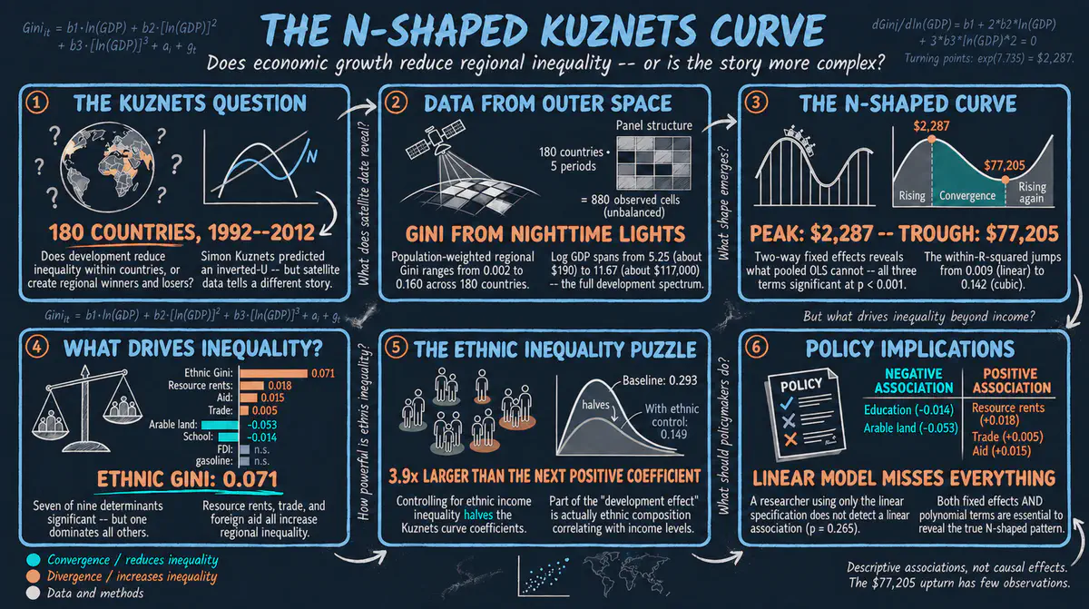
Replicating the N-shaped Kuznets curve with panel data fixed effects in Python using PyFixest, from pooled OLS through two-way FE, turning point analysis, and determinants of regional inequality across 180 countries

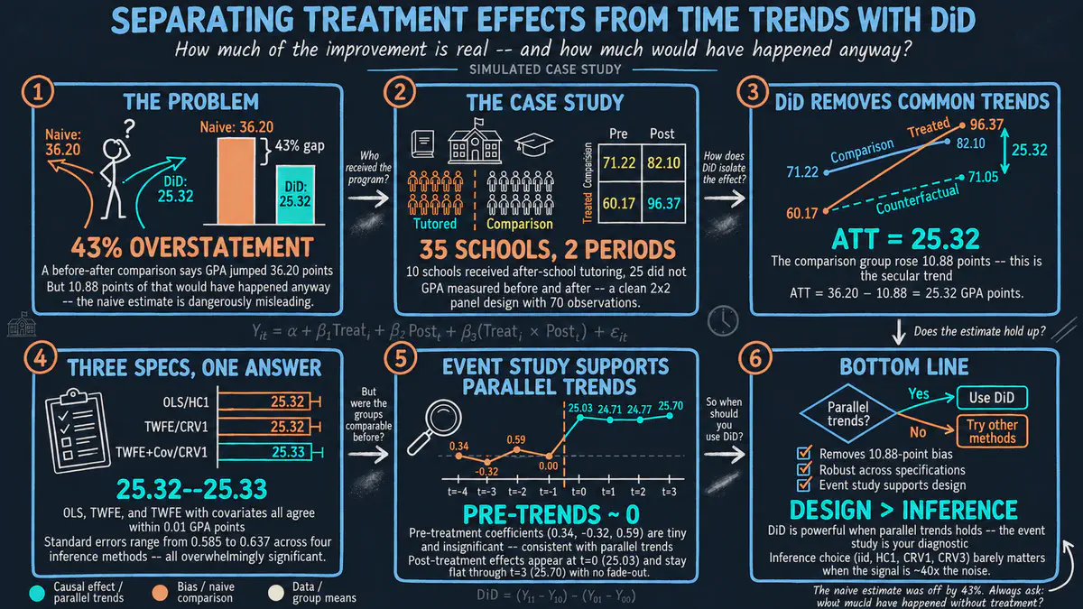
Learn Difference-in-Differences (DiD) in Python using PyFixest and Great Tables. Covers the 2x2 design, TWFE regression, inference comparison, publication-quality tables, event studies, and parallel trends testing based on Corral and Yang (2024).

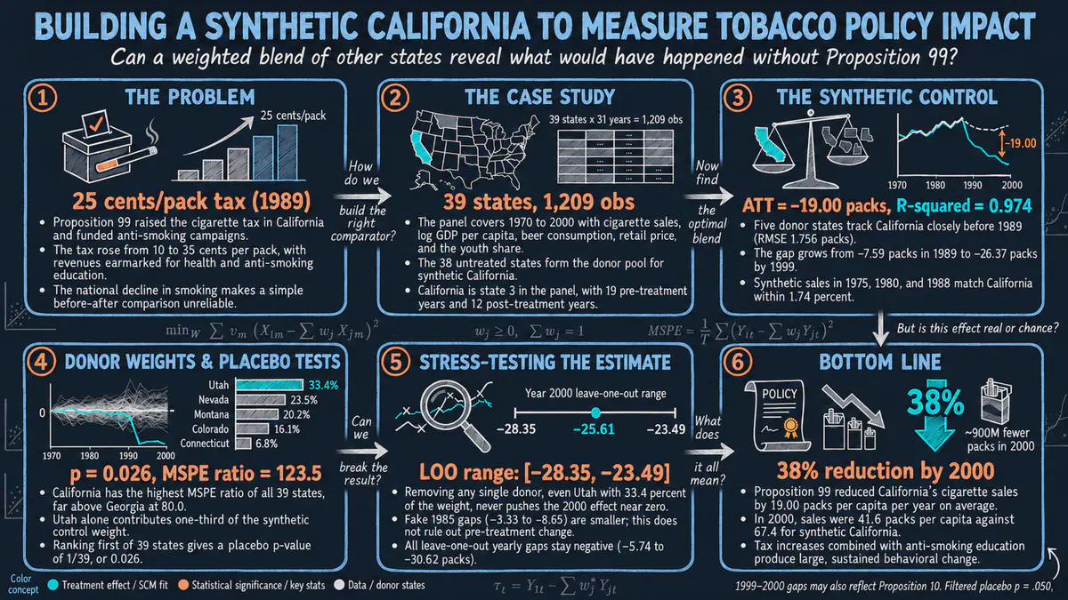
Estimate the causal effect of Proposition 99, the California tobacco control program, on cigarette sales using the synthetic control method in Stata, with in-space placebo, in-time placebo, and leave-one-out robustness tests

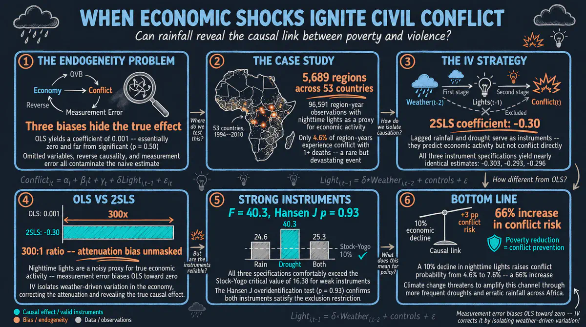
Replicate Hodler and Raschky (2014) to estimate the causal effect of economic shocks on civil conflict using 2SLS instrumental variables with panel data from 5,689 African regions

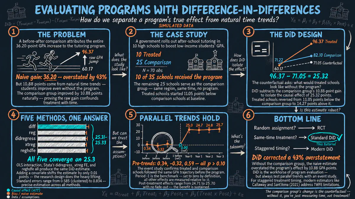
Learn Difference-in-Differences (DiD) in Stata using a case study of an after-school tutoring program. Covers the 2x2 design, TWFE regression, event studies, and parallel trends testing based on Corral and Yang (2024).

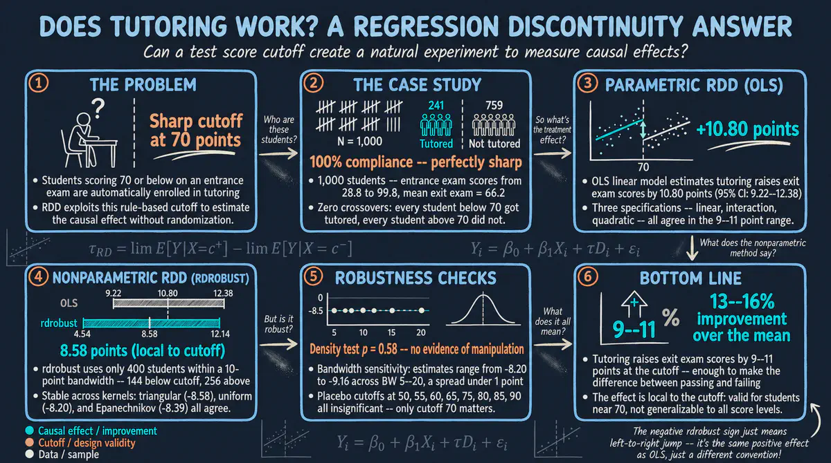
Evaluate the causal effect of a school tutoring program on student exit exam scores using sharp regression discontinuity design with parametric OLS and nonparametric rdrobust estimation in Stata

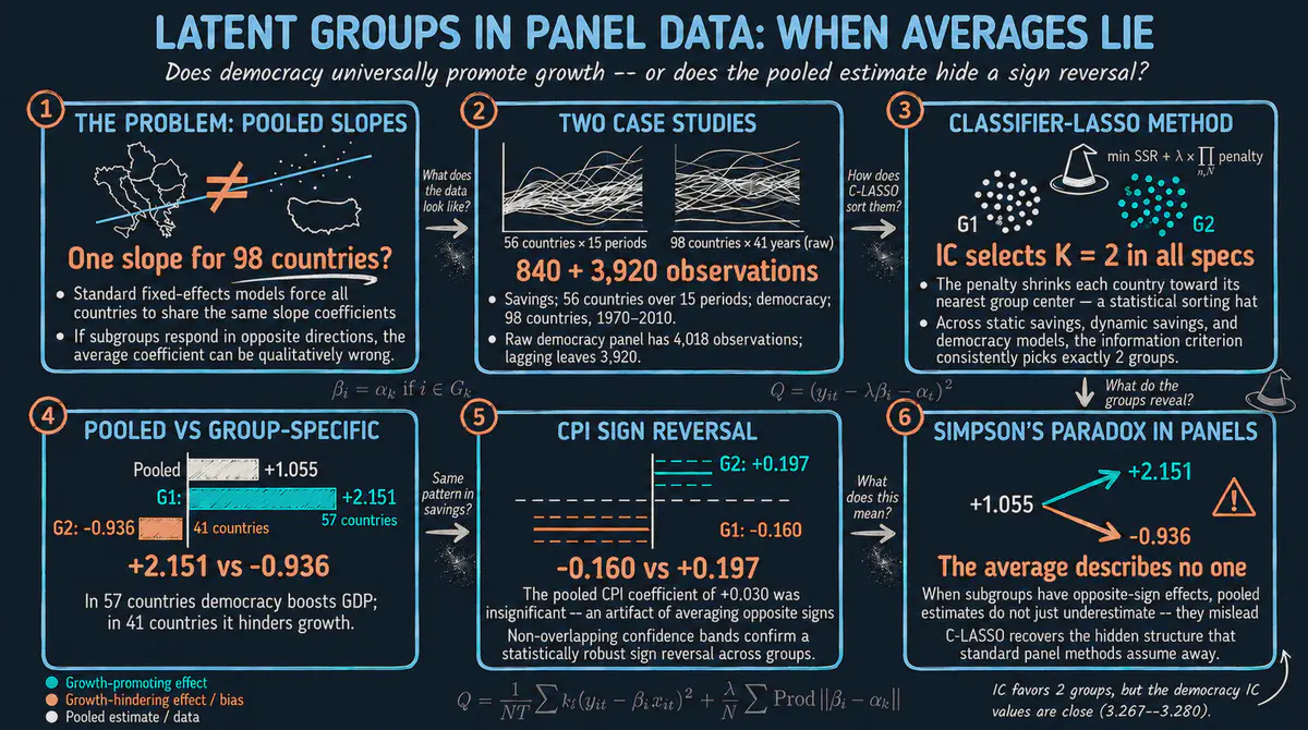
Identify latent group structures in panel data using the Classifier-LASSO method (Su, Shi, Phillips 2016), revealing that the pooled democracy-growth effect of +1.055 masks a +2.151 effect in 57 countries and a -0.936 effect in 41 countries.

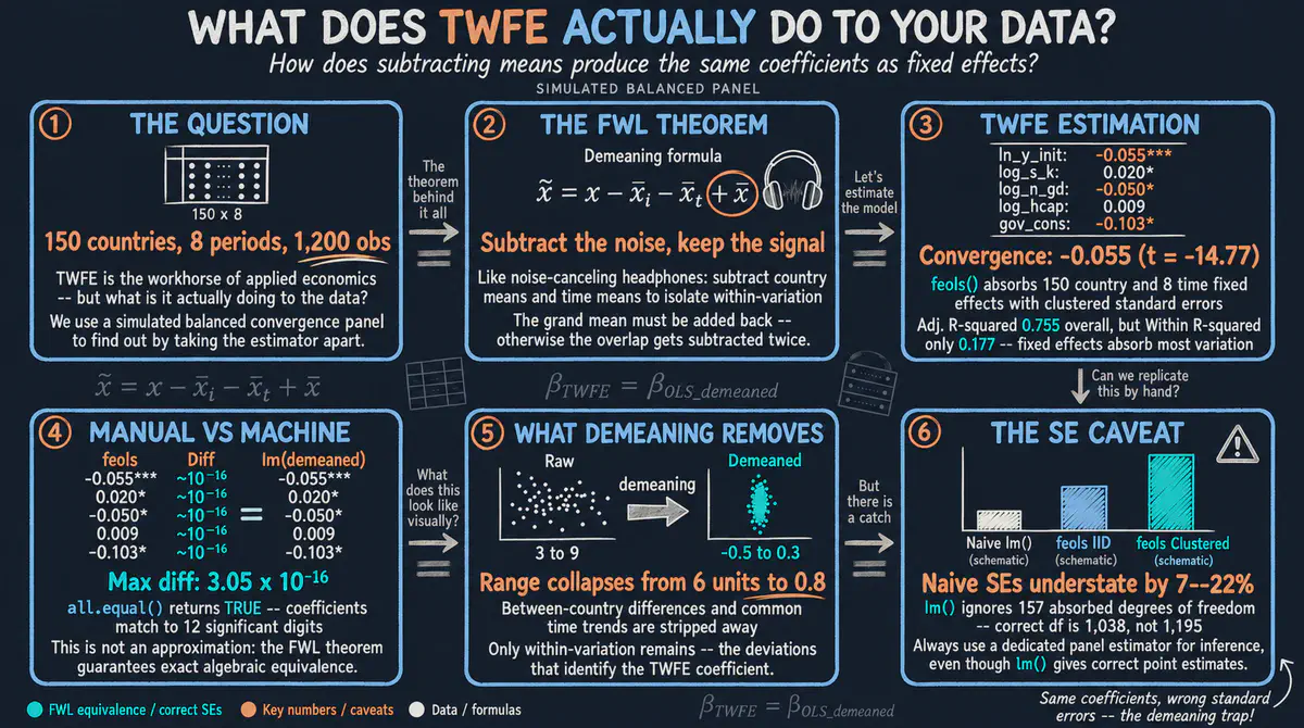
Manual demeaning vs two-way fixed effects — showing that TWFE is just OLS on demeaned data through the Frisch-Waugh-Lovell theorem, with a hands-on proof using a Barro convergence panel of 150 countries.

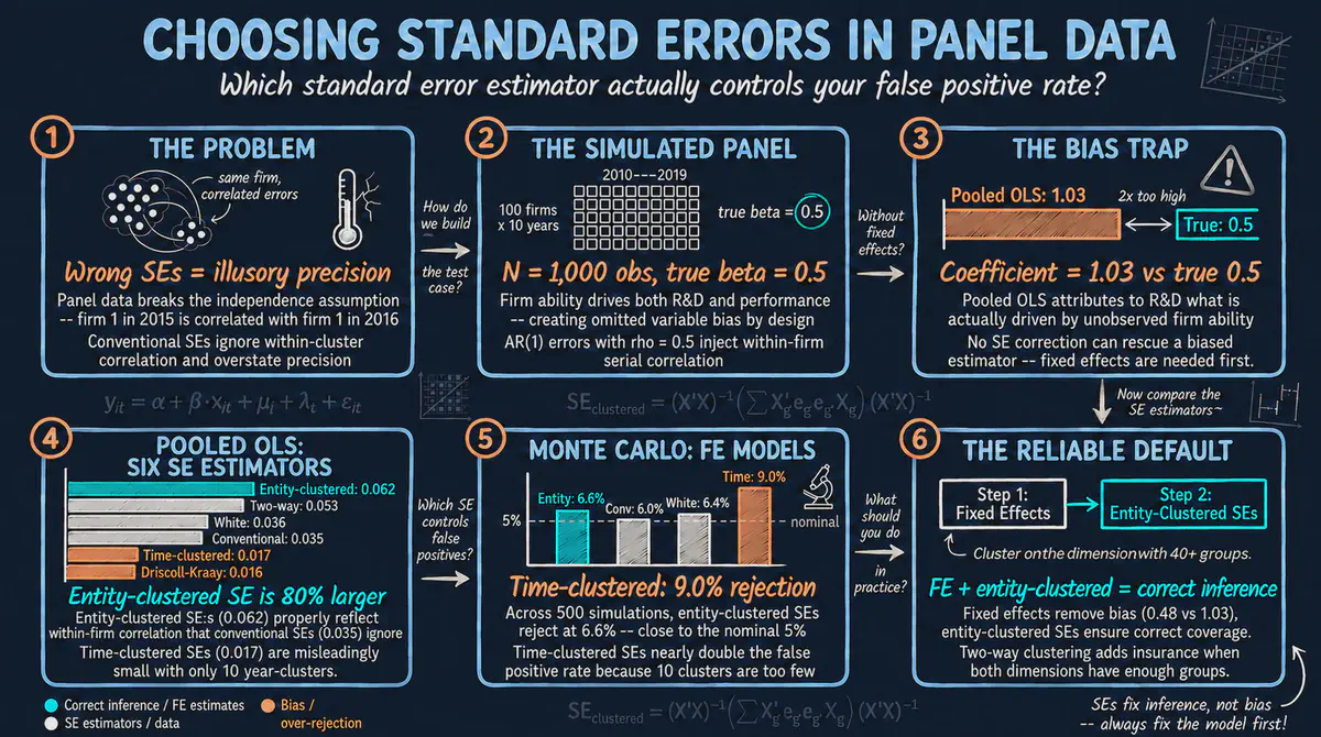
Comparing standard error estimators in panel data regressions using Python and linearmodels — from conventional to clustered, Driscoll-Kraay, and fixed effects

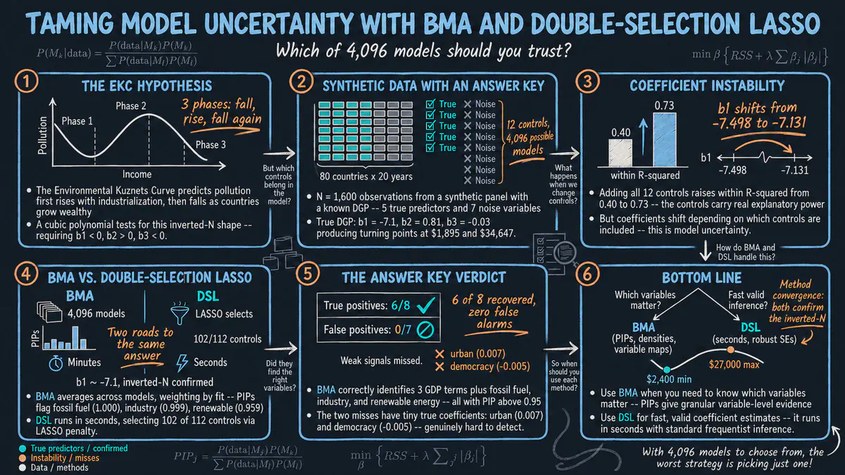
Bayesian Model Averaging and Double-Selection LASSO applied to the Environmental Kuznets Curve using synthetic panel data with a known answer key, demonstrating how both methods recover the true predictors of CO2 emissions.

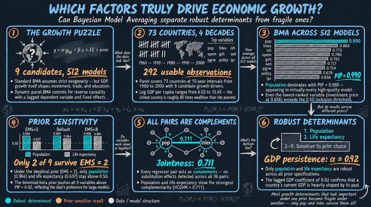
Dynamic panel Bayesian Model Averaging with the Bayesian Dynamic Systems Modeling (BDSM) R package, applied to cross-country economic growth determinants — handling reverse causality through lagged dependent variables, fixed effects, and weak exogeneity.

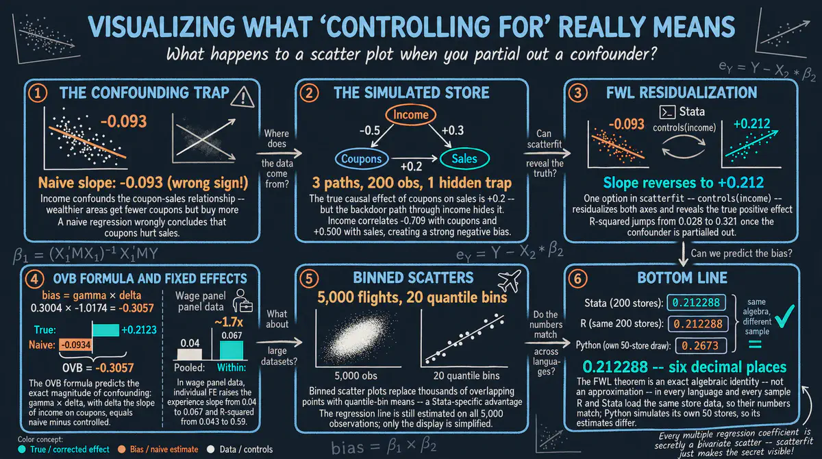
A hands-on guide to the scatterfit package in Stata — from understanding the Frisch-Waugh-Lovell theorem through simulated confounding to visualizing fixed effects in real panel data — showing what “controlling for” looks like as a scatter plot.

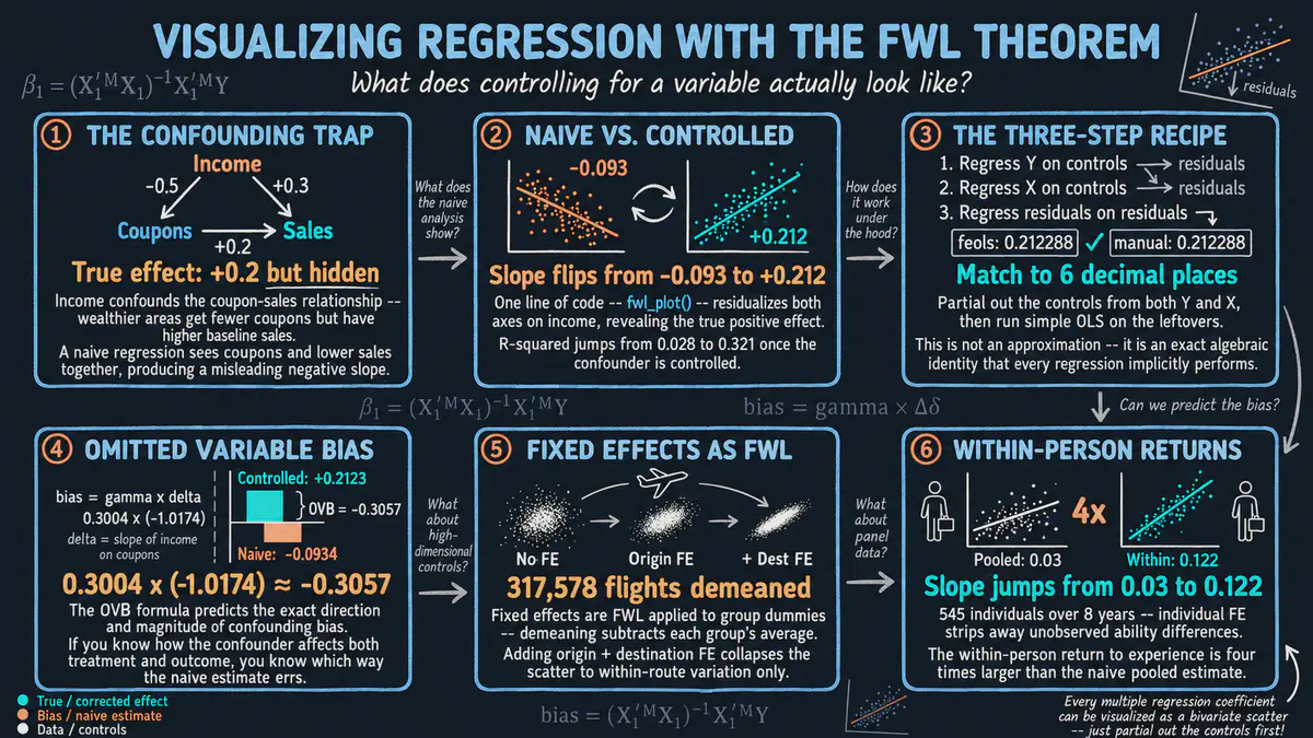
A hands-on guide to the fwlplot package in R — from understanding the Frisch-Waugh-Lovell theorem through simulated confounding to visualizing fixed effects in real panel data — showing what “controlling for” looks like as a scatter plot.

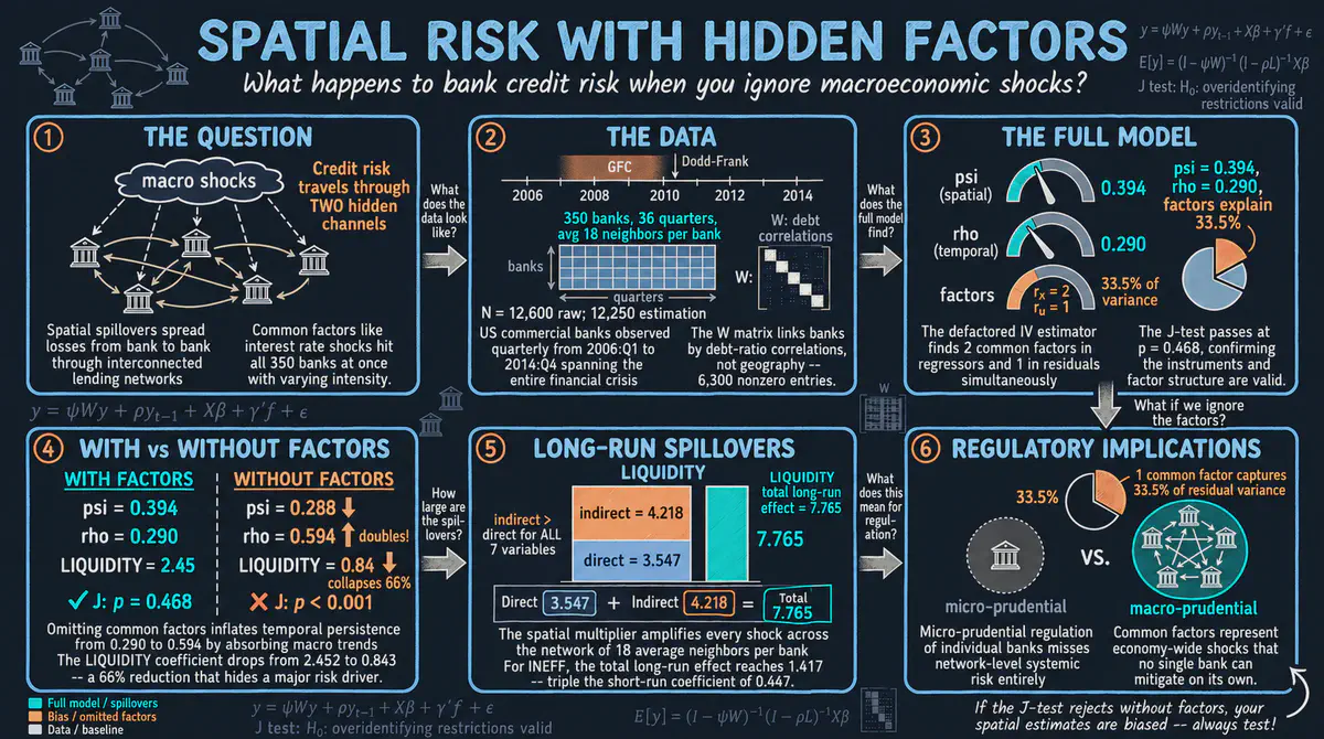
Estimate spatial dynamic panel models with unobserved common factors using the spxtivdfreg package in Stata — an IV approach that handles spatial lags, temporal persistence, endogenous regressors, and latent factors simultaneously

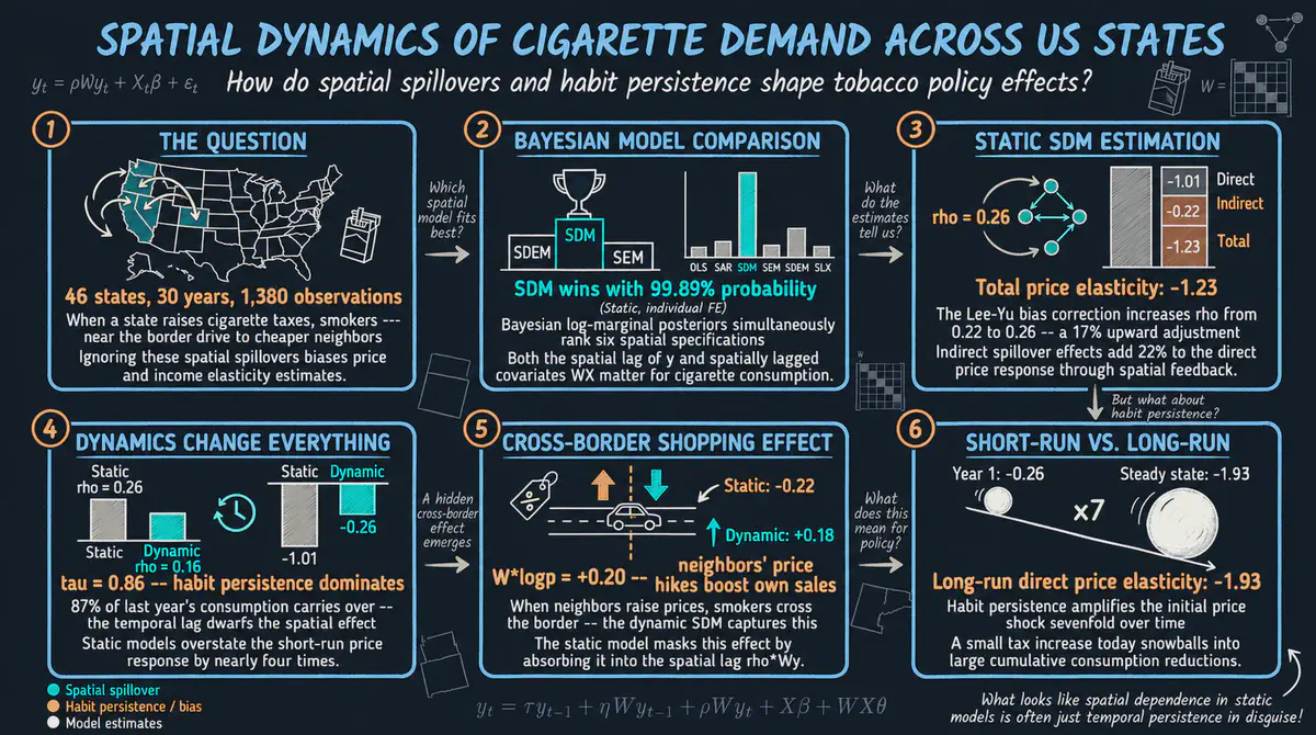
A hands-on guide to spatial panel data modeling using the SDPDmod package in R — from Bayesian model comparison through static and dynamic SAR/SDM estimation with Lee-Yu bias correction to direct, indirect, and total effect decomposition — applied to cigarette demand across 46 US states (1963–1992).

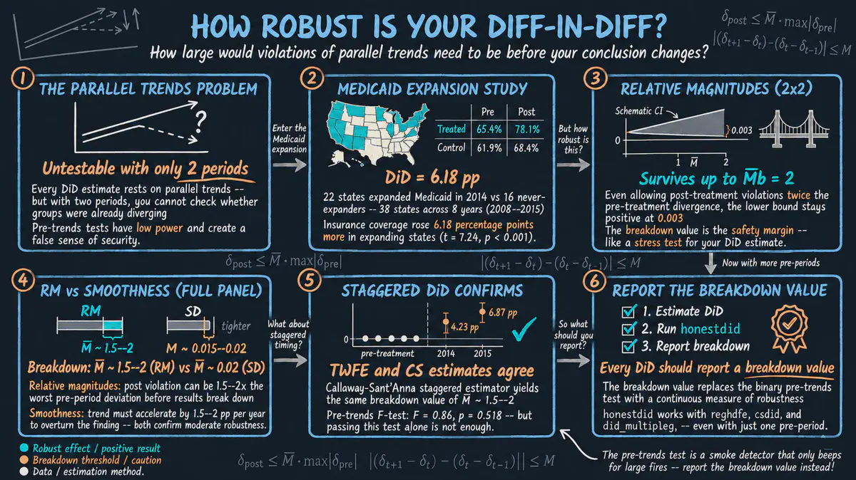
Assess how robust difference-in-differences results are to violations of parallel trends using the honestdid package in Stata, progressing from a simple 2x2 DiD to multi-period event studies with relative magnitudes and smoothness restrictions

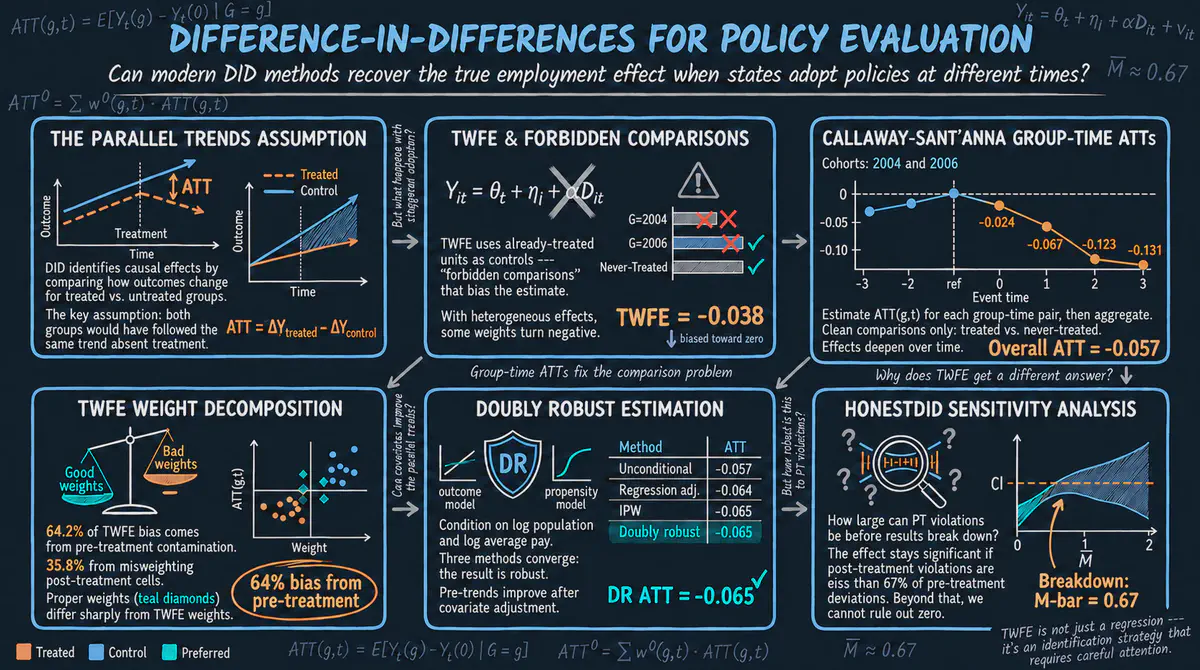
A guide to Difference-in-Differences with staggered treatment — from TWFE pitfalls through Callaway-Sant’Anna group-time ATTs, doubly robust estimation, and HonestDiD sensitivity analysis — applied to minimum wage effects on teen employment.

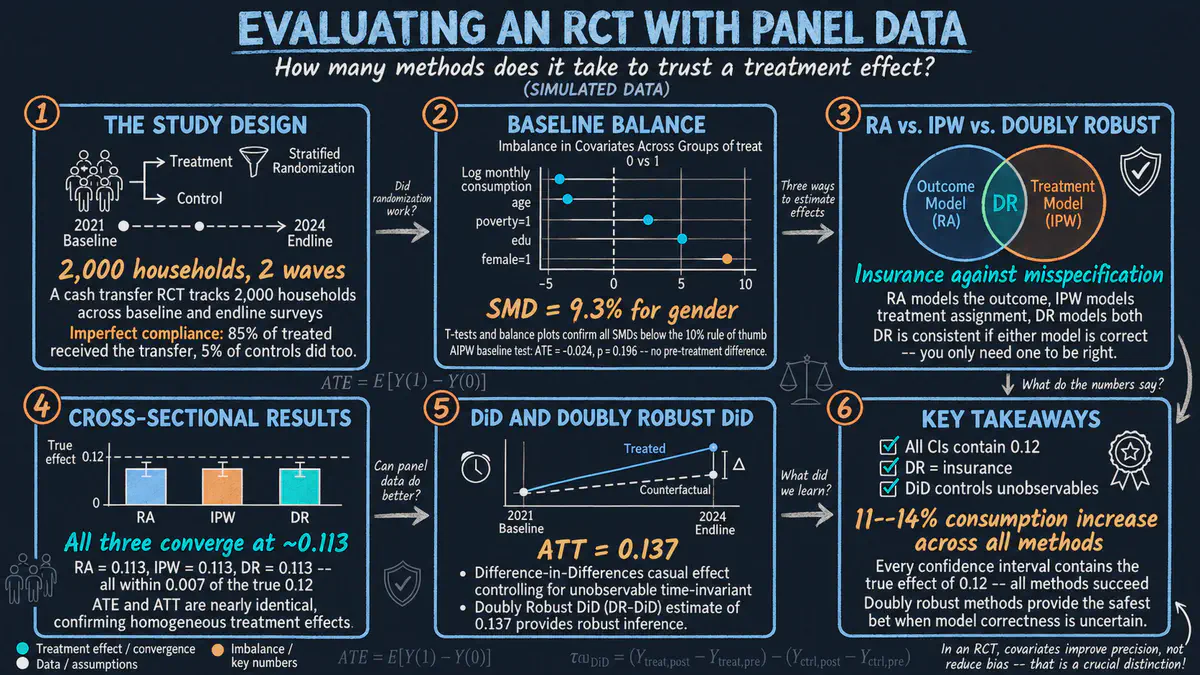
Evaluate the causal effect of a cash transfer program on household consumption using regression adjustment, inverse probability weighting, doubly robust, and difference-in-differences methods in Stata

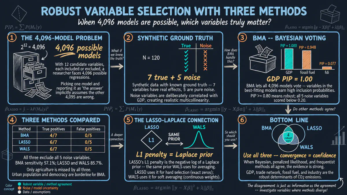
Three principled approaches to variable selection—BMA, LASSO, and WALS—applied to synthetic cross-country CO2 emissions data with known ground truth, demonstrating methodological triangulation for robust inference.

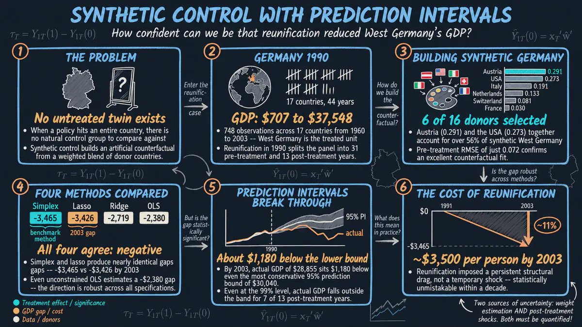
Synthetic control with prediction intervals quantifies uncertainty in Germany’s reunification GDP impact using the scpi package.

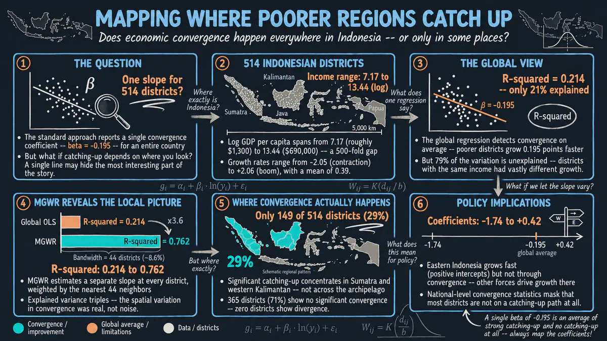
Applying Multiscale Geographically Weighted Regression (MGWR) to reveal how economic catching-up varies across Indonesia’s 514 districts, with each variable operating at its own spatial scale

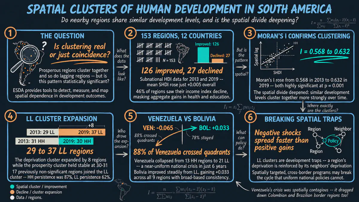
An introduction to exploratory spatial data analysis using PySAL, covering choropleth maps, spatial weights, Moran’s I, LISA clusters, space-time dynamics, and a Venezuela-Bolivia comparative analysis for 153 South American regions

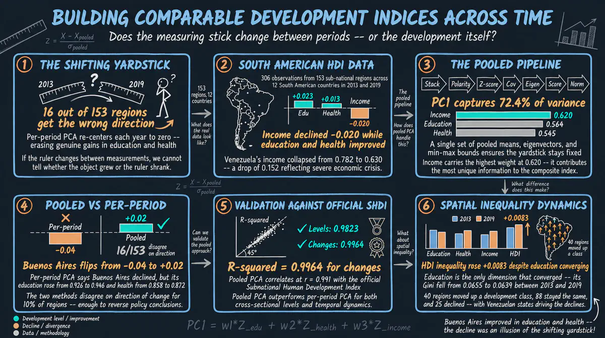
Building a comparable Human Development Index across two time periods using pooled PCA with real sub-national data for 153 South American regions, and contrasting with per-period PCA to show why pooled standardization is essential for temporal comparisons

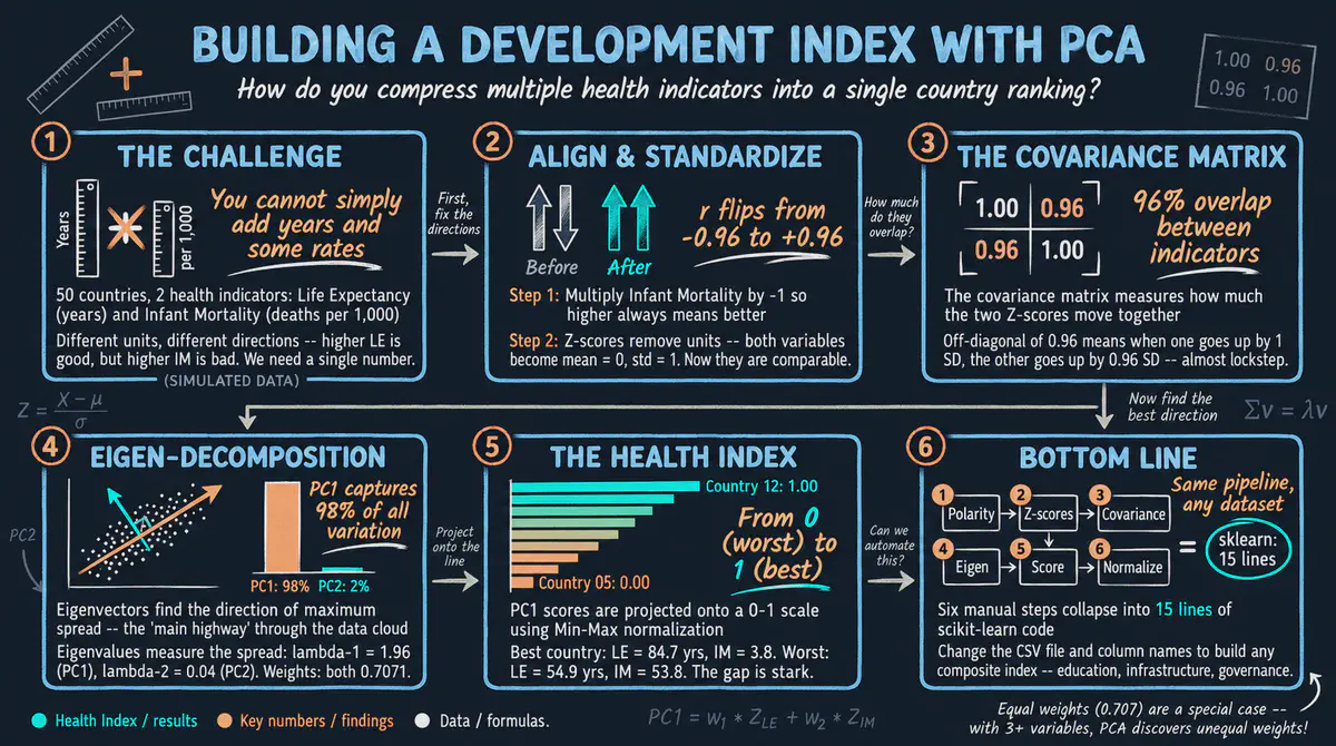
Building a composite Health Index from Life Expectancy and Infant Mortality using manual PCA with simulated data for 50 countries, then verifying against scikit-learn

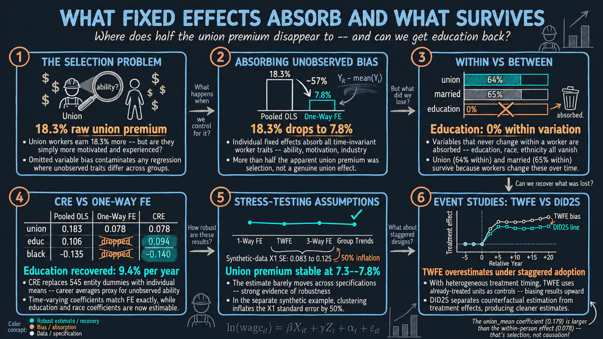
Estimating regression models with high-dimensional fixed effects using PyFixest, from simple OLS through two-way FE, instrumental variables, panel data, and event studies

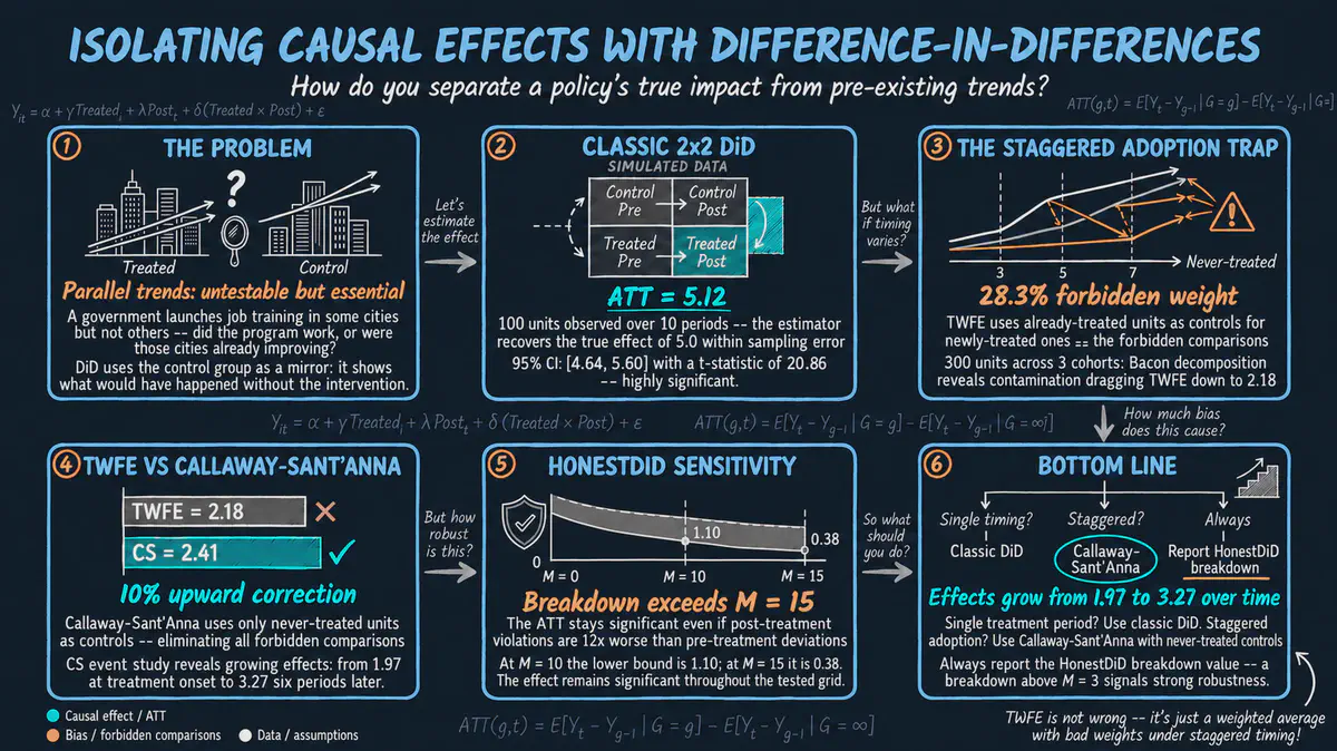
Estimating causal treatment effects using Difference-in-Differences with the diff-diff package, from the classic 2x2 design through staggered adoption with Callaway-Sant’Anna and HonestDiD sensitivity analysis

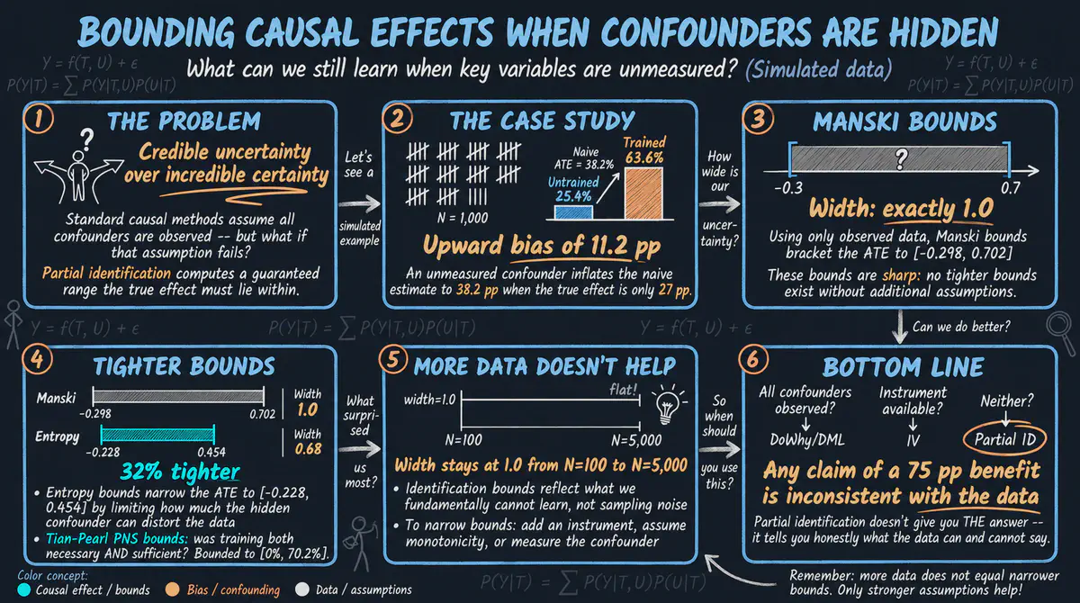
Computing causal bounds under unmeasured confounding using Manski and Tian-Pearl bounds with the CausalBoundingEngine package in Python

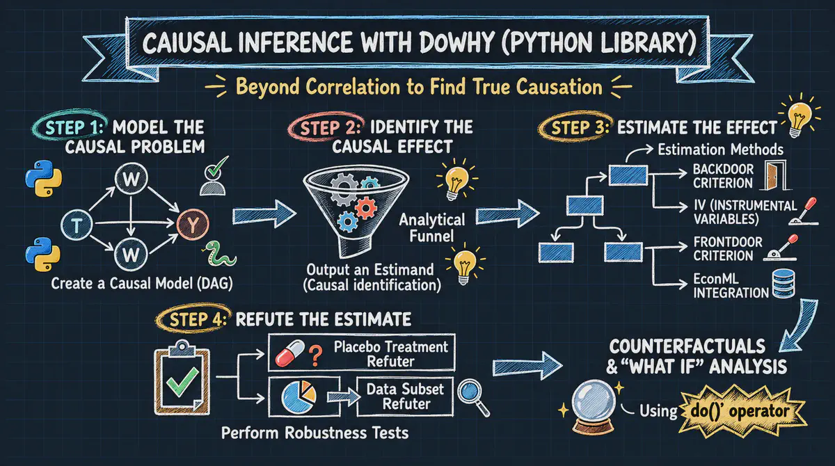
Estimating the causal effect of a job training program on earnings using DoWhy’s four-step causal inference framework with the Lalonde dataset

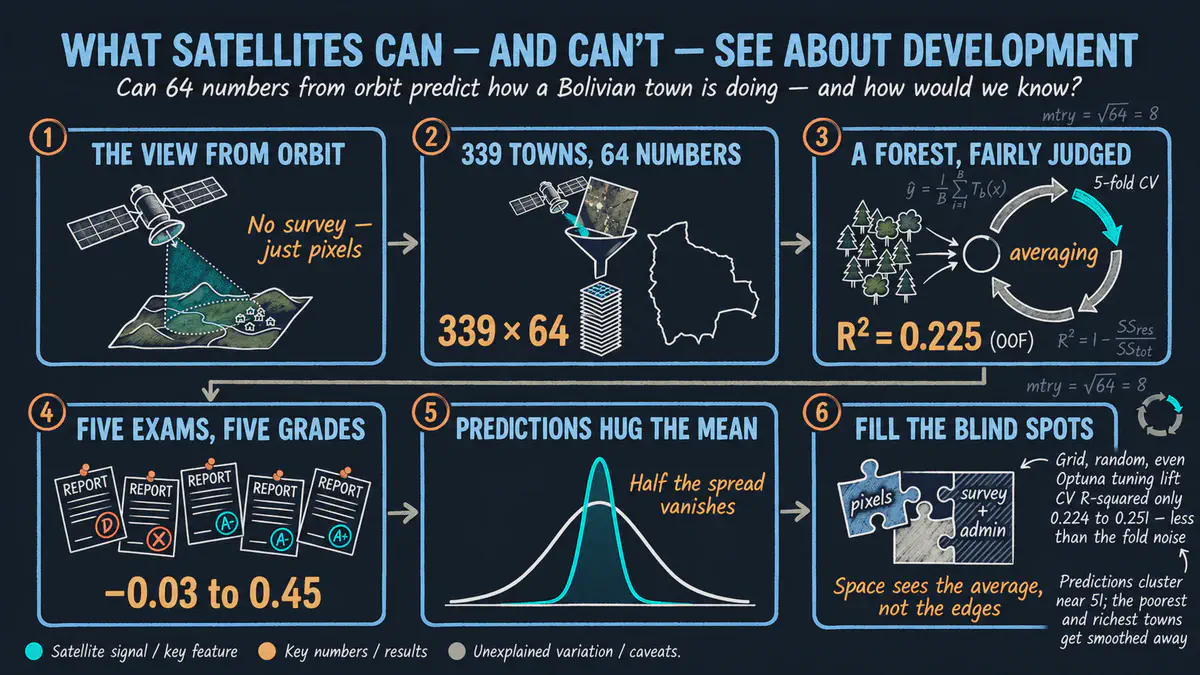
A beginner-friendly, comprehensive introduction to Random Forest regression for continuous data, evaluated end-to-end with 5-fold cross-validation and out-of-fold predictions on Bolivian satellite imagery

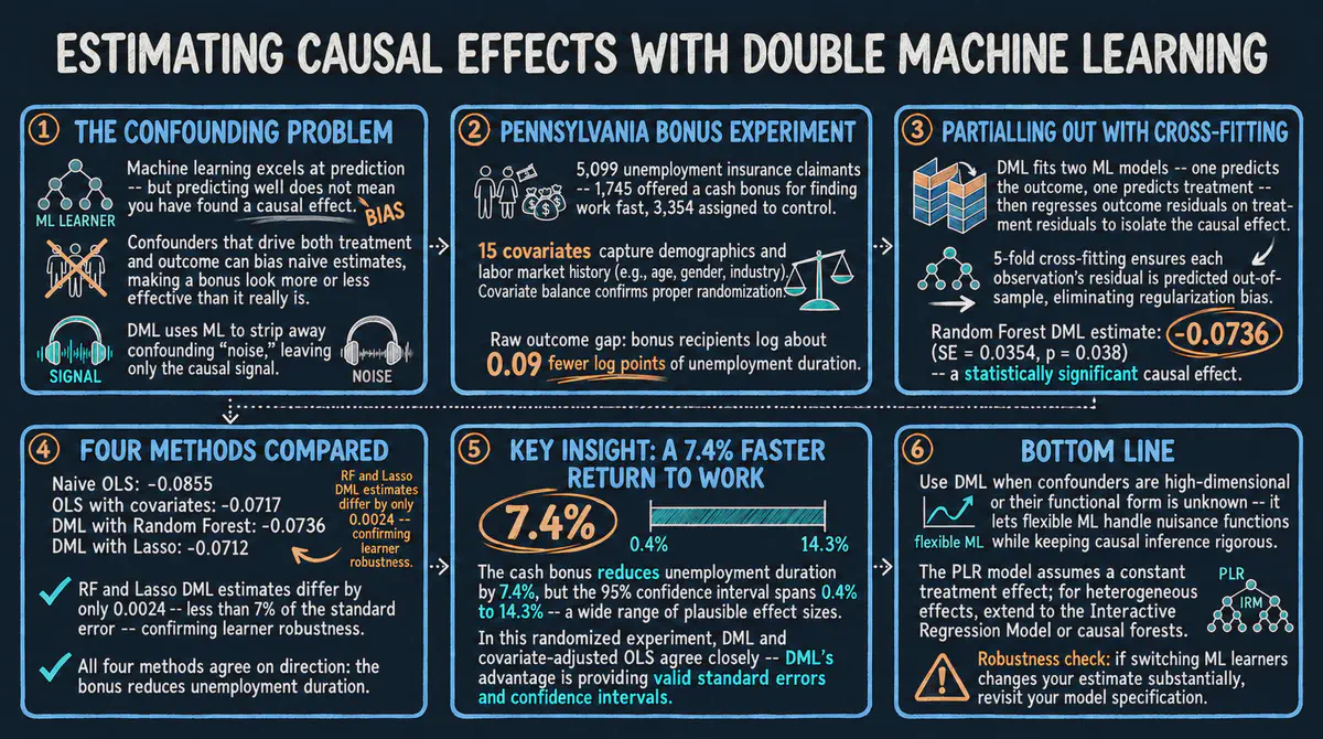
Estimating the causal effect of a cash bonus on unemployment duration using Double Machine Learning with the Pennsylvania Bonus Experiment

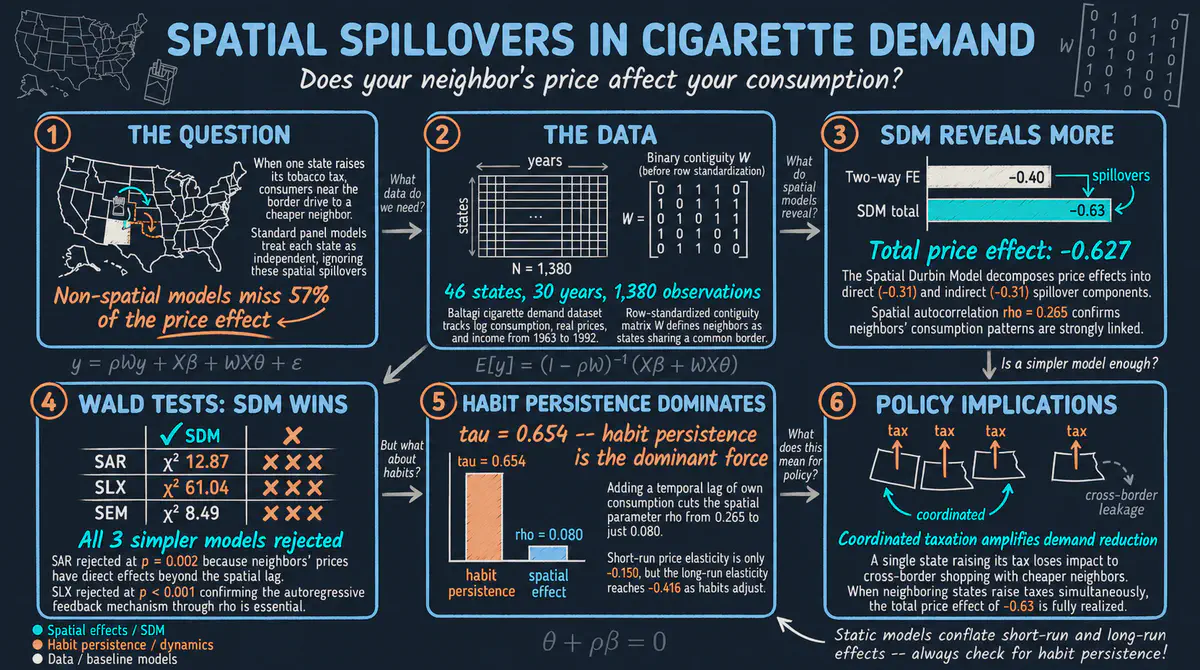
Model spatial spillovers in panel data using the Spatial Durbin Model (SDM), Wald specification tests, and dynamic extensions with the xsmle package in Stata

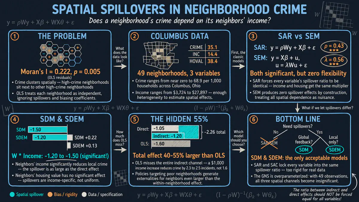
Explore the full taxonomy of cross-sectional spatial models — OLS, SAR, SEM, SLX, SDM, SDEM, SAC, and GNS — using the Columbus crime dataset in Stata, following Elhorst (2014)